Evaluation AC1-02: Difference between revisions
David.Fowler (talk | contribs) No edit summary |
m (Dave.Ellacott moved page Gold:Evaluation AC1-02 to Evaluation AC1-02 over redirect) |
||
| (5 intermediate revisions by 2 users not shown) | |||
| Line 80: | Line 80: | ||
</span> | </span> | ||
<span id="velocity profiles"> | <span id="velocity profiles"> | ||
In Figure 7, the [[#velocity profiles|velocity profiles]] at the [[# | In Figure 7, the [[#velocity profiles|velocity profiles]] at the [[Test_Data_AC1-02#EXP12 :|stations B and D]] are presented. The station B is very critical because the flow is separated or very close to the separation. The Wilcox and the Kok TNT κ-ω, and the κ-g EARSM yield the worst results. The Menter SST κ-ω and the non linear κ-ε provide a velocity profile in excellent agreement with the experimental data. At the station D the flow is attached and all the numerical results show a good agreement with the experiments. | ||
</span> | </span> | ||
The [[# | The [[Description_AC1-02#Case 4|experimental flow field]] visualization is presented in Figure 2. A triple shock wave occurs over the inner half-span of the upper surface. Outboard of this there is a single shock which provokes local separation. On the lower surface no shock waves are present, and the adverse pressure gradient and the sweep of the wing causes a deviation of the flow from the free-stream direction up to 45 o degrees. All the applied turbulence models simulate the shock wave system in a satisfactory manner, and predict the flow to separate where the three shock waves meet. The flow three dimensionality is more pronounced, especially in the outboard part of the wing, for the non linear κ-ε. As an example, the [[#flow field|flow field]] on the upper surface of the wing, as predicted by the Menter SST κ-ω turbulence model, is show in Figure 8. | ||
Satisfactory and consistent results have been presented; the more sophisticated the turbulence model the more accurate the simulation is. The numerical results have shown a reasonable agreement with the experimental data. The QinetiQ results, probably due to the modelling of the turbulent scale g and/or to the tuning of the Mach number, show in the trailing edge region of the outboard sections of the wing an excessive sensitivity to the adverse pressure gradients. Some considerations about the behaviour of the applied turbulence models can be drawn. The worst results have been provided by the standard Wilcox κ-ω model. The Spalart Allmaras, the Myong and Kasagi κ-ε, and the Kok TNT κ-ω turbulence models have shown a similar level of accuracy. The non linear κ-ε and the Menter SST κ-ω have best predicted the shock boundary layer interaction. | Satisfactory and consistent results have been presented; the more sophisticated the turbulence model the more accurate the simulation is. The numerical results have shown a reasonable agreement with the experimental data. The QinetiQ results, probably due to the modelling of the turbulent scale g and/or to the tuning of the Mach number, show in the trailing edge region of the outboard sections of the wing an excessive sensitivity to the adverse pressure gradients. Some considerations about the behaviour of the applied turbulence models can be drawn. The worst results have been provided by the standard Wilcox κ-ω model. The Spalart Allmaras, the Myong and Kasagi κ-ε, and the Kok TNT κ-ω turbulence models have shown a similar level of accuracy. The non linear κ-ε and the Menter SST κ-ω have best predicted the shock boundary layer interaction. | ||
Latest revision as of 14:59, 11 February 2017
RAE M2155 Wing
Application Challenge 1-02 © copyright ERCOFTAC 2004
Comparison of Test data and CFD
The numerical results achieved by QinetiQ for cases 2 and 4 and by CIRA for case 2 are compared to the experimental data in this section. The numerical solutions have been performed by QinetiQ using two Reynolds stress constitutive relations in combination with the scale determining equations of Kalitzin-Gould (these models can be considered a variation of the Menter SST turbulence model), and an explicit algebraic Reynolds stress model (EARSM) incorporating a variable ratio of the turbulence production to dissipation rate. The SST and EARSM solutions are nearly indistiguishable and therefore only the EARSM solution has been included in the data base.
Case 4 Flow Condition
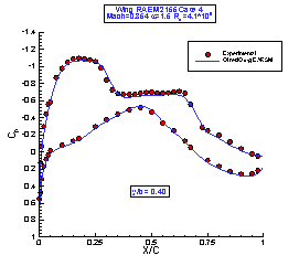
A comparison between the computed and the measured pressure coefficients, for the case 4 flow condition, is shown in Figure 3.
Figure 3: : Wing RAE M2155 Case 4 – Pressure Coefficients
The shocks location is correct, but the pressure levels in the trailing edge region on the upper surface of the wing are lower than the experimental values. This reveals a a large region of separated flow and, looking at the oil picture flows [1,2], this is consistent with the presence of a too large free stream Mach number. A better agreement with the experimental data has been achieved by using a Mach number of 0.843, 1.4% lower than the experimental value [3].
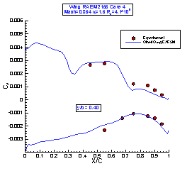
The friction coefficients are presented in Figure 4. There is a reasonable good agreement with the experimental data, though an underprediction in the trailing edge region for the more outborard section is evident.
Figure 4 : Wing RAE M2155 Case 4 : Friction Coefficients
Case 2 Flow Condition
Results achieved by QinetiQ and CIRA for the case 2 flow conditions are presented in the Figures 5-8.
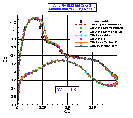
The pressure coefficient at four stations along the span is shown in Figure 5. The comparison with the experimental data is generally good.The QinetiQ results match well the shock location, but an underprediction of the pressure in the trailing edge region of the outborad sections and the presence of an unwanted separation is evident. It is worth noting that the results achieved by QinetiQ, due to a excessively long inflow section of the mesh, correspond to a Mach number slightly above the nominal. The CIRA results achieved by using several turbulence models lie in a narrow band. In the sections where the shock boundary layer interaction is stronger, the non linear κ-ε and the SST Menter κ-ω models better predict the shock location and the pressure recovery behind the shock and in the trailing edge zone.
The Friction coefficients are shown at two spanwise stations are shown in Figure 6.
Figure 5 : Wing RAE M2155 Case 2 – Pressure Coefficients
Figure 6 : Wing RAE M2155 Case 2 – Friction Coefficients
The comparison with the experimental data is globally satisfactory also if the measurements are available only at few points. The QinetiQ results, mainly at the more outboard section, underpredict the experimental data and do not compare very well.
The highest values of the friction coefficient are provided by the Wilcox κ-ω and the lowest by the Myong-Kasagi and by the non linear κ-ε models. The Wilcox κ-ω predicts the flow to separate more outboard than all the other models, and provides the smallest flow separated zone.
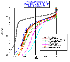
Figure 7 : Wing RAE M2155 Case 2 : Velocity profiles at station B (left) and at station D (right)
In Figure 7, the velocity profiles at the stations B and D are presented. The station B is very critical because the flow is separated or very close to the separation. The Wilcox and the Kok TNT κ-ω, and the κ-g EARSM yield the worst results. The Menter SST κ-ω and the non linear κ-ε provide a velocity profile in excellent agreement with the experimental data. At the station D the flow is attached and all the numerical results show a good agreement with the experiments.
The experimental flow field visualization is presented in Figure 2. A triple shock wave occurs over the inner half-span of the upper surface. Outboard of this there is a single shock which provokes local separation. On the lower surface no shock waves are present, and the adverse pressure gradient and the sweep of the wing causes a deviation of the flow from the free-stream direction up to 45 o degrees. All the applied turbulence models simulate the shock wave system in a satisfactory manner, and predict the flow to separate where the three shock waves meet. The flow three dimensionality is more pronounced, especially in the outboard part of the wing, for the non linear κ-ε. As an example, the flow field on the upper surface of the wing, as predicted by the Menter SST κ-ω turbulence model, is show in Figure 8.
Satisfactory and consistent results have been presented; the more sophisticated the turbulence model the more accurate the simulation is. The numerical results have shown a reasonable agreement with the experimental data. The QinetiQ results, probably due to the modelling of the turbulent scale g and/or to the tuning of the Mach number, show in the trailing edge region of the outboard sections of the wing an excessive sensitivity to the adverse pressure gradients. Some considerations about the behaviour of the applied turbulence models can be drawn. The worst results have been provided by the standard Wilcox κ-ω model. The Spalart Allmaras, the Myong and Kasagi κ-ε, and the Kok TNT κ-ω turbulence models have shown a similar level of accuracy. The non linear κ-ε and the Menter SST κ-ω have best predicted the shock boundary layer interaction.
Figure 8 : Wing RAE M2155 Case 2 – Pressure distribution and skin friction lines
(upper surface)
The flow investigated is strongly shear dominated, does not involve significant stress anisotropy and does not show strong streamline curvature or rotational effects. An SST scheme is therefore sufficient and a complexity of an EARSM or of a non linear eddy viscosity formulation is not necessary for the simulation of this kind of flow.
© copyright ERCOFTAC 2004
Contributors: Pietro Catalano - CIRA; QinetiQ
Site Design and Implementation: Atkins and UniS


