UFR 2-06 Evaluation: Difference between revisions
David.Fowler (talk | contribs) (New page: {{UFR|front=UFR 2-06|description=UFR 2-06 Description|references=UFR 2-06 References|testcase=UFR 2-06 Test Case|evaluation=UFR 2-06 Evaluation|qualityreview=UFR 2-06 Quality Review|bestp...) |
m (Dave.Ellacott moved page Gold:UFR 2-06 Evaluation to UFR 2-06 Evaluation over redirect) |
||
| (5 intermediate revisions by 3 users not shown) | |||
| Line 1: | Line 1: | ||
{{UFR|front=UFR 2-06|description=UFR 2-06 Description|references=UFR 2-06 References|testcase=UFR 2-06 Test Case|evaluation=UFR 2-06 Evaluation|qualityreview=UFR 2-06 Quality Review|bestpractice=UFR 2-06 Best Practice Advice|relatedACs=UFR 2-06 Related ACs}} | {{UFR|front=UFR 2-06|description=UFR 2-06 Description|references=UFR 2-06 References|testcase=UFR 2-06 Test Case|evaluation=UFR 2-06 Evaluation|qualityreview=UFR 2-06 Quality Review|bestpractice=UFR 2-06 Best Practice Advice|relatedACs=UFR 2-06 Related ACs}} | ||
| Line 17: | Line 16: | ||
== Comparison of CFD calculations with Experiments == | == Comparison of CFD calculations with Experiments == | ||
The results of numerical simulations were compared with experimental data using the interferometric measurements of flow fields and the pressure distribution on the blade surface for the inlet angle | The results of numerical simulations were compared with experimental data using the interferometric measurements of flow fields and the pressure distribution on the blade surface for the inlet angle β<sub>1</sub> = 70.7 deg and for the exit Mach numbers M<sub>2is</sub> = 0.716 and 1.198. The corresponding values of the loss coefficient are given in Tab.3. | ||
<center>[[Image:U2-06d32_files_image018.jpg]] [[Image:U2-06d32_files_image020.jpg]]</center> | <center>[[Image:U2-06d32_files_image018.jpg]] [[Image:U2-06d32_files_image020.jpg]]</center> | ||
| Line 23: | Line 22: | ||
<center>a) Spalart-Allmaras model b) Menter SST modified model</center> | <center>a) Spalart-Allmaras model b) Menter SST modified model</center> | ||
<center>Fig.6 Mach number isolines for M<sub>2is</sub | <center>Fig.6 Mach number isolines for M<sub>2is</sub>=0.716</center> | ||
The Mach number isolines obtained for turbulent flow using the Spalart-Allmaras model and the Menter SST modified model is shown for the subsonic regime (M<sub>2is</sub | The Mach number isolines obtained for turbulent flow using the Spalart-Allmaras model and the Menter SST modified model is shown for the subsonic regime (M<sub>2is</sub>=0.716) in Fig.6 and for the transonic regime (M<sub>2is</sub>=1.198) in Fig.7. | ||
The qualitative comparison of numerical results with the density isolines given in Figs. 2 and 3 shows a good agreement for both turbulence models including the region of the sonic line, the recompression region, and the downstream part with the shock wave structure for the transonic case. | The qualitative comparison of numerical results with the density isolines given in Figs. 2 and 3 shows a good agreement for both turbulence models including the region of the sonic line, the recompression region, and the downstream part with the shock wave structure for the transonic case. | ||
<center>[[Image:U2-06d32_files_image022.jpg]] [[Image:U2-06d32_files_image024.jpg]]</center> | <center>[[Image:U2-06d32_files_image022.jpg]] [[Image:U2-06d32_files_image024.jpg]]</center> | ||
| Line 37: | Line 34: | ||
<center>a) Spalart-Allmaras model b) Menter SST modified model</center> | <center>a) Spalart-Allmaras model b) Menter SST modified model</center> | ||
<center>Fig.7 Mach number isolines for M<sub>2is</sub | <center>Fig.7 Mach number isolines for M<sub>2is</sub>=1.198</center> | ||
The corresponding pressure distribution along the blade surface is given for the Mach number M<sub>2is</sub | The corresponding pressure distribution along the blade surface is given for the Mach number M<sub>2is</sub>=0.716 in Fig.8 and for the Mach number M<sub>2is</sub>=1.198 in Fig.9. | ||
| Line 47: | Line 44: | ||
<center>[[Image:U2-06d32_files_image026.jpg]]</center> | <center>[[Image:U2-06d32_files_image026.jpg]]</center> | ||
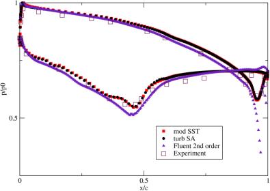
<center>Fig.8 Pressure distribution for M<sub>2is</sub>=0.716</center> | |||
| Line 55: | Line 50: | ||
<center>[[Image:U2-06d32_files_image028.jpg]]</center> | <center>[[Image:U2-06d32_files_image028.jpg]]</center> | ||
<center>Fig.9 Pressure distribution for M<sub>2is</sub>=1.198</center> | |||
| Line 63: | Line 56: | ||
From the comparison of numerical and experimental results, following comments can be concluded: | From the comparison of numerical and experimental results, following comments can be concluded: | ||
a) Isolines of the Mach number computed using in-house codes are very similar to density isolines obtained by optical measurements for both flow regimes. The FLUENT 5.0 code is not able to capture the reflected shock waves downstream the sonic line because the non-reflection boundary conditions are not implemented in the code; | |||
b) Distribution of pressure along the blade surface obtained by the in-house codes corresponds very well to experimental data in both flow regimes. The pressure distribution obtained by the FLUENT code disagrees with experimental data near the trailing edge for M<sub>2is</sub><nowiki>=0.716;</nowiki> | |||
c) The calculated energy losses obtained for M<sub>2is</sub><nowiki>=1.198 are in all the predictions lower than those for M</nowiki><sub>2is</sub><nowiki>=0.716. Values of the loss coefficient obtained for inviscid flow are naturally lower than corresponding values for turbulent flow. The main source of energy losses in the transonic regime is the existence of shock waves and therefore the values of the loss coefficient determined for inviscid flow are substantially higher than for the subsonic case. The Spalart-Allmares model and the modified SST model give the loss coefficient approximately 20% lower than experimental data for both flow regimes. </nowiki> | |||
d) The used turbulence model is not essential for capturing of flow field in the blade cascade. But for appropriate description of important phenomena of the transonic flow through the blade cascade, the prediction of the shock wave pattern and their interaction with boundary layers is crucial. The effect of the laminar/turbulent transition is important rather in the subsonic case. | |||
<font size="-2" color="#888888">© copyright ERCOFTAC 2004</font><br /> | <font size="-2" color="#888888">© copyright ERCOFTAC 2004</font><br /> | ||
| Line 79: | Line 72: | ||
{{UFR|front=UFR 2-06|description=UFR 2-06 Description|references=UFR 2-06 References|testcase=UFR 2-06 Test Case|evaluation=UFR 2-06 Evaluation|qualityreview=UFR 2-06 Quality Review|bestpractice=UFR 2-06 Best Practice Advice|relatedACs=UFR 2-06 Related ACs}} | {{UFR|front=UFR 2-06|description=UFR 2-06 Description|references=UFR 2-06 References|testcase=UFR 2-06 Test Case|evaluation=UFR 2-06 Evaluation|qualityreview=UFR 2-06 Quality Review|bestpractice=UFR 2-06 Best Practice Advice|relatedACs=UFR 2-06 Related ACs}} | ||
Latest revision as of 19:45, 11 February 2017
Flow around (airfoils and) blades (transonic)
Underlying Flow Regime 2-06 © copyright ERCOFTAC 2004
Evaluation
Comparison of CFD calculations with Experiments
The results of numerical simulations were compared with experimental data using the interferometric measurements of flow fields and the pressure distribution on the blade surface for the inlet angle β1 = 70.7 deg and for the exit Mach numbers M2is = 0.716 and 1.198. The corresponding values of the loss coefficient are given in Tab.3.
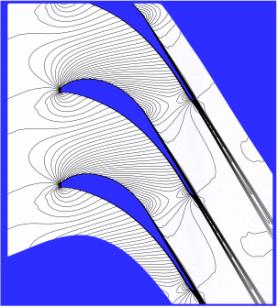
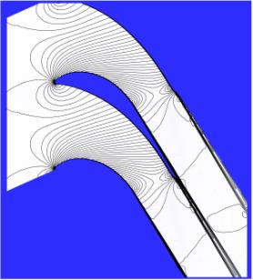
The Mach number isolines obtained for turbulent flow using the Spalart-Allmaras model and the Menter SST modified model is shown for the subsonic regime (M2is=0.716) in Fig.6 and for the transonic regime (M2is=1.198) in Fig.7.
The qualitative comparison of numerical results with the density isolines given in Figs. 2 and 3 shows a good agreement for both turbulence models including the region of the sonic line, the recompression region, and the downstream part with the shock wave structure for the transonic case.
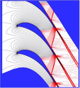
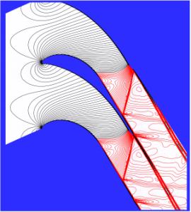
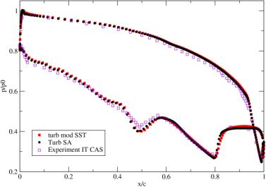
The corresponding pressure distribution along the blade surface is given for the Mach number M2is=0.716 in Fig.8 and for the Mach number M2is=1.198 in Fig.9.
From the comparison of numerical and experimental results, following comments can be concluded:
a) Isolines of the Mach number computed using in-house codes are very similar to density isolines obtained by optical measurements for both flow regimes. The FLUENT 5.0 code is not able to capture the reflected shock waves downstream the sonic line because the non-reflection boundary conditions are not implemented in the code;
b) Distribution of pressure along the blade surface obtained by the in-house codes corresponds very well to experimental data in both flow regimes. The pressure distribution obtained by the FLUENT code disagrees with experimental data near the trailing edge for M2is=0.716;
c) The calculated energy losses obtained for M2is=1.198 are in all the predictions lower than those for M2is=0.716. Values of the loss coefficient obtained for inviscid flow are naturally lower than corresponding values for turbulent flow. The main source of energy losses in the transonic regime is the existence of shock waves and therefore the values of the loss coefficient determined for inviscid flow are substantially higher than for the subsonic case. The Spalart-Allmares model and the modified SST model give the loss coefficient approximately 20% lower than experimental data for both flow regimes.
d) The used turbulence model is not essential for capturing of flow field in the blade cascade. But for appropriate description of important phenomena of the transonic flow through the blade cascade, the prediction of the shock wave pattern and their interaction with boundary layers is crucial. The effect of the laminar/turbulent transition is important rather in the subsonic case.
© copyright ERCOFTAC 2004
Contributors: Jaromir Prihoda; Karel Kozel - Czech Academy of Sciences