UFR 4-13 Evaluation

Front Page

Description

Test Case Studies

Evaluation

Best Practice Advice

References

Compression of vortex in cavity

Underlying Flow Regime 4-13               © copyright ERCOFTAC 2004

Evaluation

Comparison of CFD calculations with Experiments

The calculations presented here were performed using STAR-CD, a transient, multi-phase and multidimensional CFD code, now widely used for internal combustion engine simulations. They were performed by Imperial College within a European Research program. Validation was based on the IMFT square piston test case.

The first simulations presented here where performed with an operational guillotine, producing a compression ratio of about 10. The fine 2D grid of 8000 cells was applied with RNG k-ε and the Launder Gibson-Reynolds Stress Transport Model (LG-RSTM). Previous results obtained with coarse mesh with RNG turbulence model are also presented.

During the intake at 90 Crank Angle Degrees (CA) After Top Dead Centre (ATDC), the axial velocity using the RNG k-ε model, is qualitatively close to the experimental data. During the compression and especially at the end of the compression (at 270 CA. ATDC) when of the tumble vortex breaks down, The RNG k-ε shows a poor comparison with experimental data. Finer meshing produces better prediction.

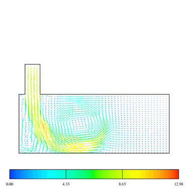
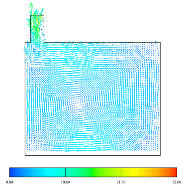
The flow field predicted with the Launder Gibson Reynolds Stress Transport Model (LG-RSTM) are shown in the Figures 8, 9 and 10. The predicted axial velocity during the intake (at 90 deg ATDC) is less accurate than k-epsilon results. On the contrary, during compression, the LG-RSTM model shows better results than the k-epsilon, cf. Figure 7. A fairly large discrepancy is observed near the wall in the case of the Reynolds stress model; this problem is shared by the other numerical results but to a lesser extent. This defect occurs also during the intake and the compression strokes.

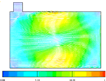
LES calculations were carried out with an open guillotine at a compression ratio with a longer intake duct and random stream-wise fluctuations imposed in the inlet. A coarse 3D grid of about 90K cells was used for a one-cycle simulation. Undeniably, LES calculations give better agreement with experiments during both the intake and the compression even with coarse mesh and a single cycle, see Figures 6,7 and 11.

Figure (8) - LGRST Predicted flow field and axial velocity with

compression tumble CR=10 and at 90 ATDC

 

Figure (9)- LGRST Predicted flow field and axial velocity

with compression tumble CR=10 and at 270 ATDC

 

Figure (10)- LGRST Predicted flow field

with compression tumble CR=10 and at 310 ATDC

Fig (11-a)

Fig (11-b)

Fig (11) Predicted flow field in longitudinal mid-plane during induction and exhaust for non compressing tumble case CR = 4, obtained using low Reynolds number subgrid model

More recently, LES developments were reported in Moureau et al. 2004 and Devesa et al. 2004 with the square piston as a validation test case. The unstructured parallel AVBP CFD code was used to predict cyclic variability occurring in Internal Combustion (IC) engines.

An Arbitrary Lagrangian Eulerian (ALE) method was implemented with 2nd order finite volume and 3rd order finite element convective schemes with moving solid boundaries. LES modelling validation was performed by comparing simulations results obtained on 2D and 3D meshes and using two convective schemes with experimental data on the square piston experiment.

The simulations clearly showed that even if the mean flow is essentially 2D during the intake phase, only a full 3D simulation is able to capture the breakdown of the tumble during piston compression as shown in Figure 12.

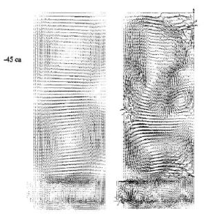
The simulations also showed that using the 3rd order TTGC (a finite element two-step Taylor-Galerkin convective scheme) , allowed for a given mesh resolution, to resolve more flow details near the cut-off scale than a 2nd order centred Lax-Wendroff type scheme, a definitive advantage for LES simulations. The mean velocity profiles obtained by phase averaging six consecutive 3D engine cycles with a standard Smagorinsky LES turbulence model combined to wall laws and using a LW scheme showed encouraging reproduction of mean experimental profiles ( cf. Figure 13).

At 90°CA BTDC

at TDC

Figure 12: mean velocity profiles at the compression phase, Moureau et al. 200

Figure 13: instantaneous velocity fields of the compression, 45° Crank Angles (CA) Before TDC (BTDC), obtained with Lax-Wendroff (left) and TTGC (right) schemes on 2D meshes. The velocity normalization is the same. (Moureau et al. 2004)

© copyright ERCOFTAC 2004

---

Contributors: Afif Ahmed - RENAULT

Front Page

Description

Test Case Studies

Evaluation

Best Practice Advice

References