UFR 3-04 Evaluation
Laminar-turbulent boundary layer transition
Underlying Flow Regime 3-04 © copyright ERCOFTAC 2004
Evaluation
Comparison of CFD calculations with Experiments
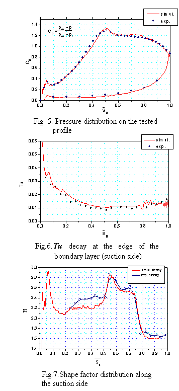
Comparison of experimental results with CFD calculation was performed for the steady case only. The analysis concerns: pressure coefficient Cp, distribution of the freestream turbulence intensity Tu at the edge of boundary layer on the suction side and distributions of integral parameters and friction coefficient (Elsner at al, 2001).
Fig.5 presents the pressure coefficient Cp distribution around the profile. The pressure coefficient Cp is defined as
where: p01 is inlet total pressure, p2 is exit static pressure, p is static pressure

On the suction side the flow accelerates sharply and reaches the minimum of pressure for S/Sg =0.5, then the moderate deceleration is observed. For the pressure side one may observe almost constant velocity of the flow for most of the surface and then the flow gradually accelerates towards the trailing edge. For both pressure and suction sides one may observe a good agreement between experimental results and the calculations. Numerical simulation confirms even the small deceleration zone close to the leading edge on the suction side, which is due to blade nonlinearity in the region where the circular leading edge matches the further part of the profile. Such phenomena are very common specially for HP blades where thick leading edge is applied to ensure a proper heat distribution or for incorporation of cooling system. Numerical simulation confirms also the small separation region just after the pressure peak, where constant pressure level is visible with consecutive laminar bubble recovery region. From Fig.5 it is seen the acceleration in the first part of the blade associated with the 350% decrease of pressure coefficient and then only 50% pressure coefficient increase due to deceleration in the rear part.
Fig.6 presents distribution of freestream turbulence intensity Tu at the edge of boundary layer on the suction side. The boundary layer thickness was determined at the place where velocity was 0.98 of the freestream velocity. The data presented confirm that the decaying tendency of Tu for both experiment and simulation cases was similar what means that freestream turbulence was well modeled by the solver. Some discrepancy, seen close to the leading edge of the blade (Ss=0-0.05), is due to overproduction of turbulent kinetic energy, the inherent phenomenon of k-ε model, not sufficiently dumped by the Durbin treatment (Durbin, 1996). The same problem was reported by Vicedo at all (2003) in the simulation of the flow around semi-circular leading edge plate (ERCOFTAC T3L test case).

The most credible evaluation of the numerical procedures may be obtained from comparison between numerically and experimentally determined characteristics of the boundary layer. The results concerning boundary layer parameters obtained from steady calculations (e.g. integral parameters, shape factor, skin friction coefficient) confirm good agreement with the experimental data for most of the profile surface. For the shape factor (Fig. 7) the only difference between numerics and experiment is visible for the acceleration part of the profile where modeling approach underpredicts the experimental results. The most important region is the rear part of the profile, where boundary layer development which decides about the magnitude of losses, is captured well by the simulation. After the local increase of shape factor (Ss=0.55-0.65), (which is probably due to small separation) the transition begins beyond Ss=0.71 point. The conclusion concerning the separation is based only on the result of the oil visualization shown in Fig. 2, as the shape factor and Cf do not capture well this phenomenon. Close to the trailing edge from Ss=0.85 a purely turbulent boundary layer is present.
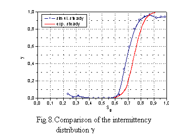
The key variable used in describing boundary layer during transition from laminar to turbulent flow is the intermittency factor γ. Moreover, most of the empirical transitional models are based on extensive use of this parameter. Fig. 8 presents the intermittency distribution along the blade surface, both for experiment, and for the numerical simulation, where experimental results were obtained based on hot-wire signal differentiation and smoothing as described by Hedler and Keffer (1974). In the intermittent region between Ss=0.61-0.85, turbulent spots form and grow as they travel downstream. It is well known, and observed also in other data that some turbulent activity, and so the increase of intermittency is observed prior to the change of general flow properties indicated by rise of skin friction and drop of shape factor. The same behaviour of boundary layer is also observed in the analysed case. One can notice some delay in the numerical results, obtained with PUIM procedure, in spite of the consistence in shape factor distributions. It could be concluded that, because the external turbulence is of the order of 1%, and additionally Tolmien-Schlichting waves were not identified on the time traces before the intermittency starts to rise, the transition process is of the bypass type.

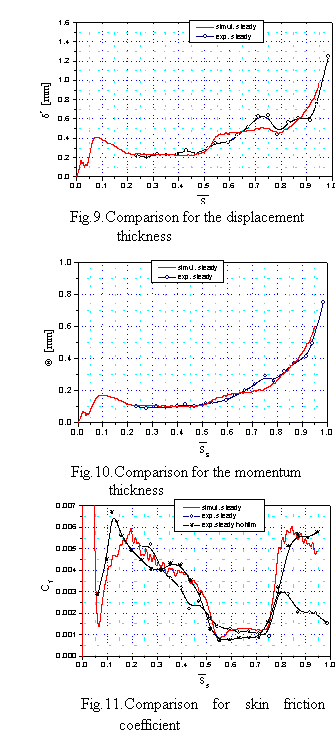
Distributions of integral parameters δ* and θ (Fig.9 and 10) also show sufficient agreement. Some differences emerge for displacement thickness especially in the region between the pressure peak and transition zone, where modeling approach first overpredicts and then underpredicts the experimental results. This inconsistency has no distinct influence on the shape factor H because θ shows similar but less distinct shape. The most important is however, the coincidence of momentum thickness between experimental and numerical data as θ is a good indicator of friction loses generated in the boundary layer. Fig.11 shows calculated and measured friction coefficients Cf along the blade. The measured Cf distribution is presented based on hot-wire data. On the rear part of the blade the calculated friction coefficient follows closely the experimental data and again the transition zone is captured very well. Some discrepancy is observed in the region from Ss=0.3 to 0.5 at acceleration part of the blade where calculations overpredict the experiment that agrees with the behavior which was already discussed on the occasion of shape factor evolution. Additionally, the unexplained difference at the turbulent region (Ss>0.75) is visible, where the calculated friction coefficient is much higher than the measured one. The black line shows the distribution of skin friction calculated from hot-film measurements. These data should be treated only as qualitative information as they are calculated based on quasi shear stresses, and one can compare here only the shape of its distribution. This distribution fits much better the numerical data than the one obtained from hot-wire measurements especially in the region of turbulent boundary layer. However, this problem is far from beginning fully understood and one should not draw rush conclusion about the validity of hot-wire measurements.
© copyright ERCOFTAC 2004
Contributors: Andrzej Boguslawski - Technical University of Czestochowa
