AC 6-10 Best Practice Advice
Axial compressor cascade
Application Challenge 6-10 © copyright ERCOFTAC 2004
Best Practice Advice
Best Practice Advice for the AC
Key Fluid Physics
Description of Application Challenge
- ECAV2-V2 high subsonic compressor cascade
- Wind tunnel measurements at DFVLR Braunschweig
- AGARD WG18 test case
- Inlet Mach numbers 0.3-0.9
- Flow turning 50o
- High incidence/stall – choke
- Variation of streamtube
DOAPs
- Exit Mach number, M2
- Exit flow angle, α2
- Pressure Loss, ζ
- Blade surface pressure distributions, Cp
- Pressure loss across wake, ω
Boundary layer velocity profiles on suction surface
Flow Physics
- Stagnation point at leading edge
- Initial laminar region is followed by transition
- Turbulent boundary layer thickens and eventually separates
- High turning produces strong adverse pressure gradient
- Local supersonic regions near blade surface
Underlying Flow Regimes
- Stagnation point flow (3-12)
- Laminar-turbulent boundary layer transition (3-04)
- Bypass transition on a flat plate (3-19)
- 2D boundary layers in adverse pressure gradients (3-03)
- The main focus of the UFR Best Practice Advice is on turbulence modeling. Therefore the majority of the discussion regarding the best practice advice and its consistency with the UFRs is contained in the section on physical modeling.
2. Application Uncertainities
Turbulent length scale at inlet
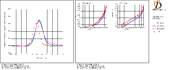
- Turbulent length scale at inlet is unknown so comparison of varying turbulent length scale at inlet was carried out (coarse mesh, k-e RNG)
- As length scale is increased:
– Higher loss and thicker wake
– Fuller velocity profiles
- Effect of length scale quantified. 5% of pitch chosen for all simulations
- UFR 3-19 indicates the importance of initial and freestream conditions for turbulent dissipation for prediction of bypass transition.

|
|
|
|
|
|
|
|
|
|
|
|
|
|
|
|
|
|
|
|
Axial variation of streamtube thickness
- Data only provides an overall value of streamtube contraction
- Two possible axial variations of streamtube were investigated:
– a) Linear variation between the inlet and exit measuring planes
– b) Constant values upstream and downstream and a linear variation between leading and trailing edges
- Option a) is more accurate and was used for all simulations
Computational Domain and Boundary Conditions
Computational domain
- One blade pitch with blade located centrally
- Axial extent -0.8 to 1.8 axial chords from leading edge
- Pseudo-2D with prescribed variation of streamtube
- Sensitivity of results to streamtube variation has been investigated
Boundary Conditions
- Inflow boundary
– fixed stagnation pressure
– Specified flow angle, total temperature
– Turbulence intensity: 5%, length scale: 5% pitch
- Outflow boundary
– Fixed static pressure adjusted to give correct inlet Mach number
- No-slip wall boundaries on blade surface
- Cyclic (periodic) boundaries pitchwise
- Symmetry planes on endwalls
Discretisation and Grid Resolution
- 2nd order discretisation (MARS) on momentum, enthalpy and turbulence
- Full central differencing used for density interpolation to cell faces
- Grid independence investigations:
– O grid around blade, H grid upstream and downstream
– 3 levels of general refinement
– Hybrid wall functions
– Additional refinement next to blade surface (Low Re, y+ ~ 1)
- Final low – Re mesh of 326 by 80 cells, with approx 25 cells in boundary layer (mesh 2).
- Near wall y+ consistent with advice given in UFR 3-03 and 3-04. Use of hybrid wall functions allows mesh refinement studies to cover entire domain, this is also recommended in UFR 3-03.
|
|
|
|
|
|
|
|
|
|
|
|
|
|
|
|
|
|
|
|
|
|
|
|
|
|
|
|
|
|
|
|
|
|
|
|
|
|
|
|
|
|
|
|
|
|
|
|
Physical Modelling
- Low Re number implementations recommended. Although hybrid wall functions were employed, improved prediction of near wall gradients can be achieved with a true low-Re mesh (y+ =1)
- K-e, Cubic k-e, Spalart-Allmaras, v2f used
- Reasonable prediction of DOAPs can be achieved with k-e, but improved loss prediction and capture of detailed flow features with more advanced models.
- UFRs 3-19 and 3-04 show that for 2-eq models, a low-Reynolds number implementation is required to have any chance of predicting transition (although their success may be coincidental). No specific transition models were incorporated in this study. UFR 3-04 states that linear eddy viscosity models usually need highly empirical transition correlations to be accurate.
- Most accurate boundary layer profiles obtained with cubic k-e. UFR 3-12 shows that v2f has been shown to give comparable results to Kato-Launder formulation and time scale bounded model for stagnation point flows. As boundary layer growth starts at the stagnation point (leading edge) v2f is more likely to accurately predict boundary layer development.
- General high overall loss despite under-prediction of exit flow angle is thought to be due to excessive turbulence in the freestream. This is strongly affected by inlet turbulent length scale. v2f gives lowest overall loss and most accurate loss levels from the suction surface towards the mid-blade passage.
|
|
|
|
|
|
|
|
|
|
|
|
|
|
|
|
|
|
|
|
|
|
|
|
|
|
|
|
|
|
Recommendations for Future Work
- Modelling of the complete range of operating points available in the test data with this range of turbulence models.
- Comparison of Kato-Launder and time scale bounded models with v2f and cubic k-ε for boundary layer development
- Running a wider range of turbulence models with different turbulent length scales at inlet.
© copyright ERCOFTAC 2004
Contributors: Michael Dickens; Alex Read - Computational Dynamics Ltd


