Premixed Methane-Air Swirl Burner (TECFLAM)

Application Challenge 2-08 © copyright ERCOFTAC 2011

In order to assess the simulation a comparison of the time averaged velocity, temperature and species distribution with experimental data is presented in this section. As mentioned before only the 30 kW case has been investigated by means of numerical simulations. A more extensive evaluation can be found in the cited references. .

Comparison of CFD Results with Experimental Data

RANS Simulations of the Isothermal and Reacting Flow

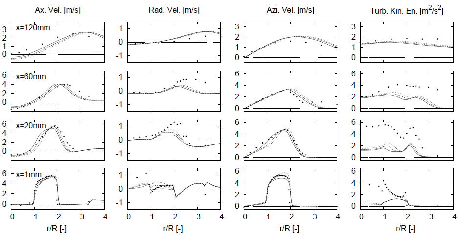
In Fig. 5.1 results of the isothermal flow field obtained with FASTEST and the k-epsilon model are shown in comparison with experimental data. Typically for this type of swirl flow, the velocity field starts to expand right after the nozzle exit, which produces a positive pressure gradient in the axial and radial direction, high enough to form a central recirculation zone as intended for flame stabilization. As will be outlined later on (see the Best Practice section) --- depending on the choice of the computational domain --- the inlet boundary conditions are crucial and not completely defined regarding the swirl intensity. Therefore isothermal RANS simulations have been used to identify the sensitivity related to this parameter. These simulations provide a cost effective way to gain knowledge for the computationally more expensive simulations dealing with the reacting case where additionally effects would overlap or compensate during such a parametric study.

Figure 5.1: Isothermal flow field. Comparison of the time-averaged axial, radial and azimuthal velocity components and the turbulent kinetic energy of the RANS simulations^[1] with experimental data (dots). Here the influence of the boundary conditions is shown using decreasing swirl (dashed --> solid). R = 15mm (radius of the bluff-body).

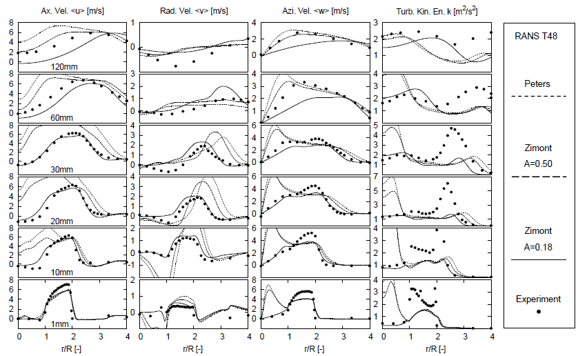
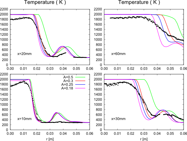
In Fig. 5.2 results of the reacting case obtained with ANSYS CFX are shown in comparison with experimental data. As mentioned before the Turbulent Flame Speed Closure model has been used to treat the chemical reaction during the simulation where a strong sensitivity related to its model coefficient can be observed. Using the Zimont correlation for the turbulent flame speed with the standard value of A=0.5 overestimates the velocity a lot. This trend was also observed in further simulations where the formulation of Peters developed for the G-equation model was applied. The reason for these deviations becomes obvious if one considers the profiles of the axial velocity at 10mm. While at higher radii within the outer shear layer the agreement is promising (as observed in the isothermal simulations)a huge acceleration occurs at the flame front because of the density change of the reaction. The turbulent flame speed that determines the flame position is too large and as a result the combustion takes place too early. As shown above, in the isothermal case of this configuration, the k-epsilon model is generally able to predict the velocity field near the nozzle exit satisfactorily and so also the shear layer, which is important for the flame stabilization. Consequently, the deviations observed so far must result from the combustion model and therewith from the turbulent flame speed. In the literature strong variations in the right choice of the modeling constant entering the correlation for the turbulent flame speed have been reported depending on the configuration investigated. For that reason a series of simulations with a different model constant have been carried out and adequate agreement could be achieved with A=0.18 which is a strong deviation from its default value A=0.5. The strong sensitivity indicates that this modeling approach is not well suited to help during the design process since even with the tuning of the flame position the scalar distribution was poorly predicted as illustrated in Fig 5.3.

Figure 5.2: Reacting flow field obtained with the RANS simulation and the turbulent flame speed closure combustion model^[2] . Influence of the correlation for the turbulent flame speed on the velocity components and turbulent kinetic energy in comparison with experimental data. R = 15mm (radius of the bluff-body).

Figure 5.3: Reacting flow field obtained with the RANS simulation and the turbulent flame speed closure combustion model^[2] . Influence of the correlation for the turbulent flame speed on the temperature ( K ) comparison with experimental data.

LES Simulations of the Isothermal and Reacting Flow

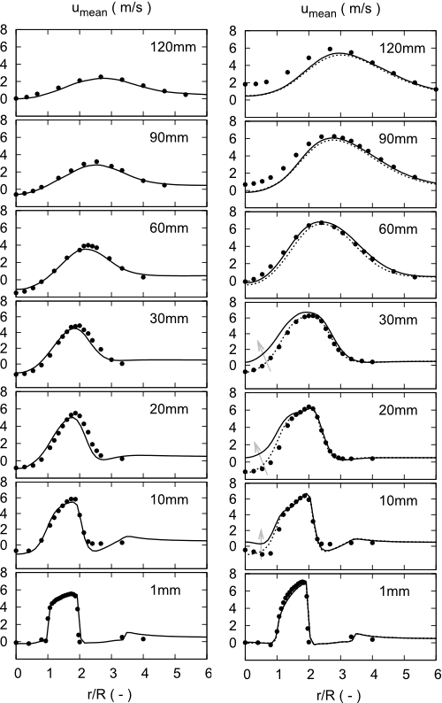
In Fig. 5.4 the simulation results of the axial velocity for the isothermal and reacting case are compared with experimental data. Overall the spreading of the turbulent swirling flow and the size and intensity of the recirculation zone are well predicted and an excellent agreement with the measurements can be observed in all axial planes for both cases. Comparing the isothermal and reacting case a strong acceleration of the velocity caused by the thermal expansion through the flame front can be observed which is accurately reproduced by the simulation.

Figure 5.4: Comparison of isothermal (left) and reacting (right) flow field. Time averaged axial velocity (u_mean) obtained by the LES^[3] using the efficiency function of Charlette et al.^[4] (solid lines) and Colin et al.^[5] (dashed lines) in comparison with experimental data (dots). R = 15mm (radius of the bluff-body).

In Fig. 5.5 the temperature and methane mass fraction are compared with experimental data. Since the flame is very sharp the distribution is almost completely caused by the flame-turbulence interaction resulting in a wide turbulent flame brush. Except that a small radial offset exists and the gradient at higher axial positions is slightly over predicted the temperature is well predicted by the simulation. The mean profile of the methane mass fraction reflects its consumption by the chemical reaction on the left and the mixing with the coflowing air on the right. At the higher axial positions the methane mass fraction exceeds the measurement indicating insufficient fuel consumption in the simulation.

Figure 5.5: Temperature (left) and methane mass fraction (right). Time averaged values obtained by the LES^[3] using the efficiency function of Charlette et al.^[4] (solid lines) and Colin et al.^[5] (dashed lines) in comparison with experimental data (dots). R = 15mm (radius of the bluff-body).

Comparing the efficiency functions (which is the main model parameter) the differences (marked with arrows in Fig. 5.4 and 5.5) between the two formulations are small and hence the model uncertainty will not influence the results crucially.

References

↑ F. Hahn, C. Olbricht, C. Klewer, G. Kuenne, R. Ohnutek, J. Janicka, in: Proc. of the ISTP19 (2008d).
↑ ^2.0 ^2.1 G. Kuenne, C. Klewer, J. Janicka, ASME Turbo Expo Conf Proc (2009) 369-381.
↑ ^3.0 ^3.1 G. Kuenne, A. Ketelheun, J. Janicka, Combustion and Flame (2011) Accepted for publication.
↑ ^4.0 ^4.1 F. Charlette, C. Meneveau, D. Veynante, Combustion and Flame 131 (2002) 159–180.
↑ ^5.0 ^5.1 O. Colin, F. Ducros, D. Veynante, T. Poinsot, Physics of Fluids 12 (2000) 1843–1863.

Contributors: Guido Kuenne (EKT), Andreas Dreizler (RSM), Johannes Janicka (EKT)
EKT: Institute of Energy and Power Plant Technology, Darmstadt University of Technology
RSM: Institute Reactive Flows and Diagnostics, Center of Smart Interfaces, Darmstadt University of Technology