UFR 3-03 Evaluation
2D Boundary layers with pressure gradients (A)
Underlying Flow Regime 3-03 © copyright ERCOFTAC 2004
Evaluation
Comparison of CFD calculations with Experiments
Several model comparison studies for this testcase have been published by Menter (1993, 1994). Additional results for this case can be found in Bardina et al. (1997) and a comprehensive validation of EARSM models in comparison with conventional two-equation is given by Hellsten and Laine (2000) and Hsu et al. (2003). As not all relevant solutions are available as data sets, the comparison is based on pictures scanned from existing articles and one set of new simulation using CFX-5. The following comparisons will be presented:
Set 1:
- SST model
- BSL model.
- k-ω model
- k-ε model
Set 2:
- SST model
- RNG k-ε model.
- SA model
- k-ε model
Set 3:
- k-ε model
- SSG model (ε-equation)
Set 4:
- Comparison from Hsu et al. (2003)
Set 5:
- Comparison by Hellsten and Laine (2000)
All simulations have been performed on low-RE grids using an integration to the surface.
The main concern with this flow is the correct prediction of the flow reversal near the wall and the proper displacement effect (reflected in the wall pressure distribution).
1.1 Results from the Present Author
Figure 4 shows a comparison of velocity profiles from the k-ε model (Jones and Launder 1972), the k-ω (Wilcox, 1993) model, the BSL and SST model (Menter, 1993, 1994) (Set 1). The simulations have been performed with the INS2D code and have been taken from Menter (1993). The velocity profiles show clearly that the k-ε is not suitable for flows with adverse pressure gradients and pressure induced separation. The model shows little sensitivity to the flow deceleration and predicts firmly attached velocity profiles. The k-ω model and the BSL model are somewhat closer to the data, but still in poor agreement with the experimental profiles. The improvement relative to the k-ε modelis a result of the improved near wall behavior of the ω-equation based models. It was shown by Wilcox (1993) that the ω-equation is superior to the ε-equation in its near wall prediction of the turbulent length-scale. The ε-equation overpredicts the near wall length-scale under adverse pressure gradient conditions, resulting in too high wall-shear stresses (Rodi and Scheuerer 1986). However, none of the three models (k-ε k-ω and BSL) accounts for the transport of the turbulent shear-stress, which is the main driving force in the momentum exchange. It was demonstrated by Johnson and King (1984) that this is important in non-equilibrium adverse pressure gradient flows. This effect is taken into account with the SST model, which results in a significantly improved representation of the experimental data.
Figure 5 shows the wall shear-stress distribution for the same turbulence models of Set 1. The results are consistent with the velocity profile prediction. However, the wall shear-stress for the k-ω and the BLS model is in better agreement with the experimental data than expected from the velocity profiles. This is a result of the proper inner scaling of these models. The only model in the comparison to reproduce the negative wall shear-stress in the separation bubble is the SST model, as expected from the velocity profiles.
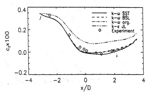
Figure 6 shows the wall pressure distribution. The flattening of the experimental pressure distribution is a result of the acceleration of the outer flow due to the separation. Clearly, the models, which do not capture the velocity profiles also fail to predict this characteristic of the pressure distribution.
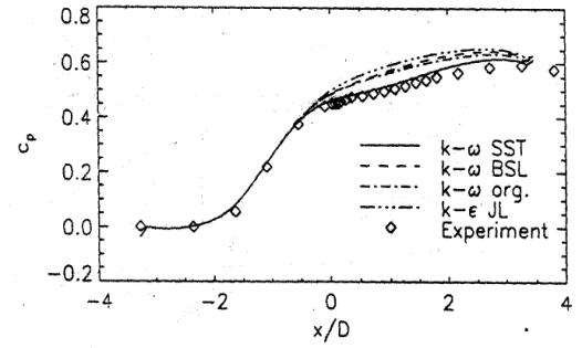
Figure 7 shows a comparison of the principal turbulent shear stress ![]() . The two sets of experimental data represent the shear-stress in the coordinate system of the wind tunnel (Carth) and in a streamline coordinate system. These systems are not identical, due to the velocity component normal to the wall. The most important profile is the first profile at (x/D=-0.091 m) as it is just upstream of the experimental separation point. The differences in the velocity profiles are a result of the differences in the turbulent shear stress. From the comparison of the results it is apparent that the tunnel-oriented shear-stress is the relevant quantity. The SST model reproduces this distribution and thereby is able to predict the correct shape of the velocity profiles. The larger the maximum of the predicted shear-stress is, the smaller is the tendency to predict the correct velocity profiles.
. The two sets of experimental data represent the shear-stress in the coordinate system of the wind tunnel (Carth) and in a streamline coordinate system. These systems are not identical, due to the velocity component normal to the wall. The most important profile is the first profile at (x/D=-0.091 m) as it is just upstream of the experimental separation point. The differences in the velocity profiles are a result of the differences in the turbulent shear stress. From the comparison of the results it is apparent that the tunnel-oriented shear-stress is the relevant quantity. The SST model reproduces this distribution and thereby is able to predict the correct shape of the velocity profiles. The larger the maximum of the predicted shear-stress is, the smaller is the tendency to predict the correct velocity profiles.
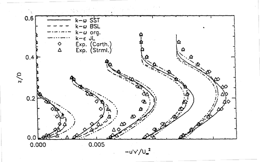
Figure 8 shows the maximum of the non-dimensional eddy-viscosity ![]() where
where ![]() is the maximum value of the eddy-viscosity profile at a given streamwise location,
is the maximum value of the eddy-viscosity profile at a given streamwise location, ![]() is the velocity at the edge of the boundary layer and
is the velocity at the edge of the boundary layer and ![]() is the displacement thickness. For equilibrium flows this value should be constant and of the order of 0.017. Figure 8 shows the reduction of this parameter due to the non-equilibrium flow predicted by the models.
is the displacement thickness. For equilibrium flows this value should be constant and of the order of 0.017. Figure 8 shows the reduction of this parameter due to the non-equilibrium flow predicted by the models.
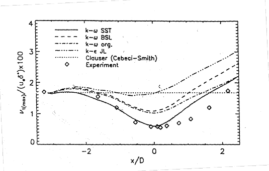
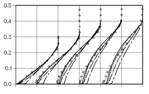
Figure 9 shows a comparison of the velocity profiles for Set 2 of the turbulence models also computed with INS2D. It shows solutions for the SST , the RNG k-ε (Yakhotet al. 1992), the Spalart-Allmaras model and the standard k-ε model. The first observation is that the k-ε RNG does not result in a significant improvement over the standard k-ε model. The second observation is that the SA model gives better results than the k-ε models and is close to the experimental data and the SST model. This explains the popularity of this model in aerodynamic solvers. Note however, that the SA model was not designed as a general-purpose model and should be used with caution in non-aerodynamic applications.
While for most industrial applications, the differences seen between the SA and the SST model for the CS0 case can be considered marginal, this is not the case for transonic flows with shock-boundary-layer interaction. These flows proved to be highly sensitive to small differences in model performance and even the marginal discrepancies seen in Figure 9 can lead to significant deviations in the pressure distribution between the two models.
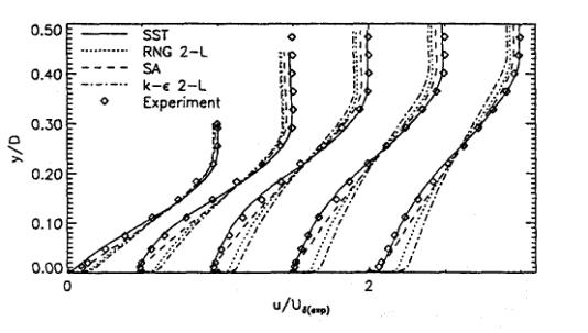
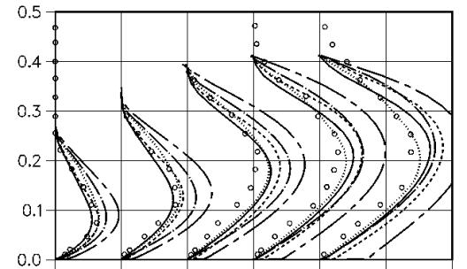
Figure 10 shows a comparison of the turbulent stress profiles for the same turbulence models of Set 2. Here the differences between the models are more visible and are consistent with the velocity profiles.
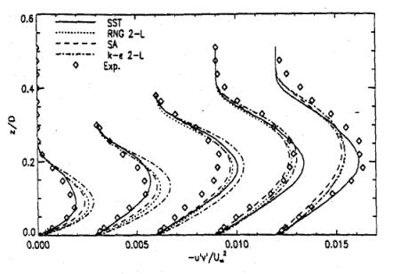
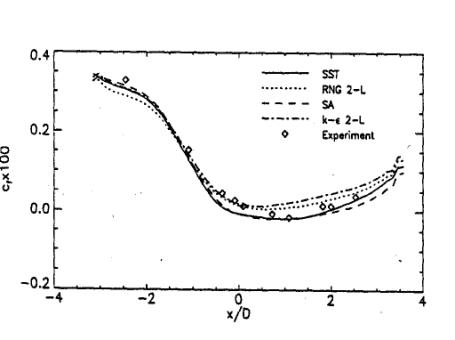
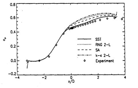
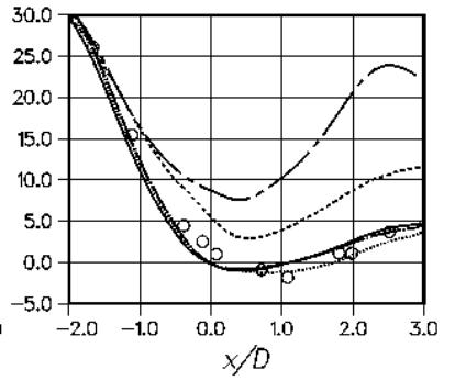
Figure 11 and Figure 12 show the wall shear-stress and the wall pressure distribution for Set 2 of turbulence models. Again, the plots are in agreement with the conclusions from the comparison of the velocity profiles.
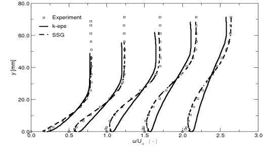
A final comparison shows the velocity profiles from the k-ε and the Spezial-Sarkar-Gatski model (Speziale et al 1991) computed with CFX-5. The last model is a Reynolds Stress model, which solves a separate transport equation for each element of the Reynolds stress tensor. The SSG model clearly gives a better representation of the displacement effect of the boundary layer and the shape of the velocity profiles than the k-ε model. Nevertheless, near the surface, the SSG model deviates from the experimental data and produces a positive wall shear-stress, as can be seen in Figure 13.
Despite the significant differences in the outer part of the boundary layer, the SSG model produces almost the same wall shear-stress as the k-ε model.
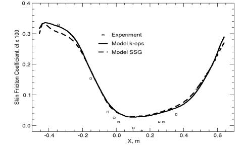
This is an example where an inconsistency is observed between the displacement effect seen in Figure 9 and the wall shear-stress distribution. The good agreement in the wall pressure distribution indicates that the displacement of the boundary layer has been computed properly, whereas the wall shear-stress distribution gives a fully attached flow field.
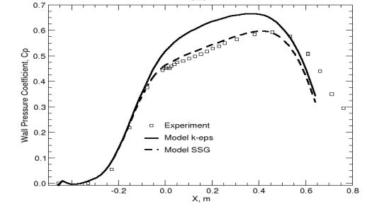
One of the reasons for the unusual behavior of the SSG model near the surface lies most likely in the use of the ε-equation in this model. While the SSG model does account properly for the transport of the shear-stresses, the ε-equation overpredicts the turbulent length-scale near the wall. This leads to a momentum exchange near the surface, which locally suppresses the separation bubble.
1.2 Results from Other Authors
The following results have been taken from Hellsten and Laine (2000) and Hsu et al. (2003) with permission from AIAA.
Figure 16 shows a comparison of velocity profiles computed with a variety of mostly non-linear stress strain models by Hsu et al. (2003). Due to the large number of curves it is difficult to see, but the agreement of the model with the data is significantly better than for the standard k-ε model.
Nevertheless, none of the models gives the correct size of the separation bubble. This can also be seen in Figure 17 and Figure 18 showing the wall shear stress and the wall pressure distributions.
Only the ω-equation based EASM approaches the zero wall shear stress limit. The other models predict no separation.
Similar conclusions can be drawn from the results of Hellsten and Laine (2000) shown in Figure 19 — Figure 22.
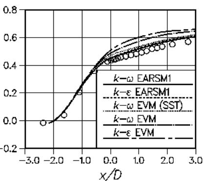
Again, the SST model is giving the best agreement with the data, closely followed by an ω-equation based EASM model.
© copyright ERCOFTAC 2004
Contributors: Florian Menter - AEA Technology


