UFR 4-05 Test Case: Difference between revisions
| Line 36: | Line 36: | ||
{| style="margin-left: 12.5pt; border-collapse: collapse; border: none" border="1" | {| style="margin-left: 12.5pt; border-collapse: collapse; border: none" border="1" | ||
| style="width: 361.9pt; border-top: .75pt; border-left: 1.5pt; border-bottom: .75pt; border-right: 1.5pt; border-color: black; border-style: solid; background: #FFFFCA; padding: 0cm 5.4pt 0cm 5.4pt" colspan="2" width="483" valign="top" | | | style="width: 361.9pt; border-top: .75pt; border-left: 1.5pt; border-bottom: .75pt; border-right: 1.5pt; border-color: black; border-style: solid; background: #FFFFCA; padding: 0cm 5.4pt 0cm 5.4pt" colspan="2" width="483" valign="top" | | ||
| Line 72: | Line 71: | ||
|} | |} | ||
== Test Case Experiments == | == Test Case Experiments == | ||
Revision as of 10:19, 31 January 2011
Curved passage flow
Underlying Flow Regime 4-05 © copyright ERCOFTAC 2004
Test Case
Brief description of the study test case
The DLR annular test cascade is a subsonic, low aspect ratio turbine stator. The stator is scaled by the factor of 2.348 and has constant hub and shroud radii. Figure 2: shows a meridional view of the geometry.

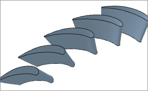
Figure 3: shows a 3D view of the blade geometry. The 3D blade coordinates can be obtained at the Institut für Antriebstechnik (Germany) (see AGARD-AR-355 for more details).

The following table gives the main dimensions of the stator.
|
Blade Geometry | |
|
Number of blades |
|
|
Chord length at hub, CH |
|
|
Chord length at midspan, CMS |
|
|
Chord length at tip, CT |
|
|
Axial chord length at midspan, CAX, MS |
|
|
Outlet flow angle reference to tangential direction, α 3 |
|
Test Case Experiments
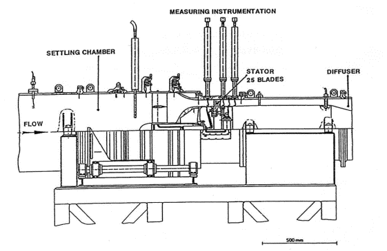
The test facility is shown in Figure 4:. It is an open loop continuously operating facility supplied with cold air.

Figure 4: Test installation (From AGARD-AR-355. « CFD Validation for Propulsion System Components», Publisher: Advisory Group for Aerospace Research & Development).
The experimental conditions are summarized in the following table.
|
Experimental conditions | |
|
Mass flow rate, m0 |
|
|
Total pressure, Pto,MS |
|
|
Total temperature, Tt0 |
|
|
Inlet flow angle, α0 (circumf.) |
|
|
Inlet flow angle, β0(Radial) |
|
|
Inlet turbulence intensity level, Tu0 |
|
|
Inlet Mach number, Ma0 |
|
|
Mean outlet Mach number, Ma3 |
|
|
Static pressure at hub, Pst,3 |
|
|
Reynolds number, Re |
|
The measurements were performed with a 5-hole probe downstream of the stator and with the three dimensional Laser-Two-Focus (3D-L2F) measuring technique inside the passage and downstream. Additionally, the upstream boundary layers were traversed using a fish-mouth Pitot probe.
The measurements were carried out on 4 planes at constant axial coordinate, one in front of the stator, 2 inside the blade passage and one downstream. These plane were located, respectively at 1.02, 0.8 0.93 and 1.4 midspan axial chord from the leading edge. Only results on the last measuring plane are discussed here.
The estimated uncertainty of the 5-hole probe data is:
- Flow angles: ±0.5 deg.
- Pressures (static and total): ±0.1 mbar
The uncertainty for the 3D Two-Focus system is:
- Velocity: ±1.5 m/s
- Flow angle: ± 0.1 to 0.2 deg.
CFD Methods
Two series of simulations on the DLR turbine stator are used in the present report. Both encompass a high number of simulations with various turbulence models. The first series came from the AGARD Advisory Report 355 whereas the second one came from new calculations performed with the FINE EURANUS/Turbo flow solver. These two series represent a total number of 29 simulations performed on this test case.
The AGARD study
The aim of the working group involved in the AGARD Advisory Report 355 was to assess the ability of CFD to predict several of the aerodynamic phenomena, which dominate the performance of turbomachines.
Numerical results of ten different flow solvers were presented in the AGARD report. Here follows a non-exhaustive list of these codes: TRANSCode, CANARI, ADPAC, RVC3D, TIP3D, TRACE-S, HAH3D, and FLOS3D. 19 simulations were performed on this test case. Among them, 8 were using an algebraic/mixing length turbulence closure model, whereas 11 calculations were using a turbulent transport model. No common grid was imposed and some participants have performed calculation with the same model on different grids (for instance TRACE-S with a k-ε turbulence model was used both with a CH and a OHHH grid).
It should be stressed that those calculations were performed in the early 90s and that those simulations are representative of the state of the art in CFD at this time.
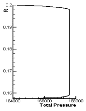
The inlet boundary condition is based on the data measured on the first plane. A profile of total pressure is imposed together with constant total temperature and angles. The total temperature is set to 306.6 K and the velocity direction is put to axial. Figure 5: shows the total pressure profile at the inlet. It must be stressed that there is uncertainties on the flow angle and velocity distributions which are were not measured at the inlet and which derived from the total pressure profile and the extrapolated pressure for the numerical experiments. At the downstream boundary the hub pressure if imposed together with a radial equilibrium.
Figure 5: Inlet Total Pressure Profile (From AGARD-AR-355. « CFD Validation for Propulsion System Components», Publisher: Advisory Group for Aerospace Research & Development).
New calculations
Ten new calculations were performed with the Code FINE(tm)/Turbo from NUMECA Int. flow solver (http://www.numeca.com). In this code, the Reynolds-averaged Navier-Stokes equations are solved with finite volume method. Central-difference is employed for the spatial discretization. A Four stage explicit Runge-Kutta scheme is applied for the temporal discretization. The multi-grid method is used combined with local time step and implicit residual smoothing to speed up the convergence.
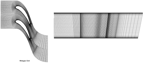
An H-O-H non-matching grid, generated with IGG/Autogrid, is used. Two grids were generated with the same number of nodes but with different cell clustering at the solid walls: 1×10⁻⁶ and 1×10⁻⁵ meter corresponding to y+ = 0.6-0.7 and y+ = 6-7, respectively. There are three blocks in the H-O-H grid, related to the inlet block, principal block, outlet block respectively, with 29×81×21 29×81×221 and 33×81×49 grid points (azimuthal × spanwise × axial). Figure 6: shows the mesh at midspan and a meridional view.
Figure 6: Mesh
Different turbulence models were applied: the Baldwin-Lomax model and four k-epsilon models: the low Reynolds Chien model, the low Reynolds Yang-Shih model, the low Reynolds Launder-Sharma model and the standard model (based on the Yang-Shih model together with an extended wall functions derived from DNS curve fitting in order to work for values of y+ greater than 20). For some turbulence models, two sets of boundary conditions for the turbulence quantities were used. The boundary condition for the turbulent kinetic energy k is set to match the turbulence intensity of the measurements (4.4%) to a constant value of 11.2 m2/s2. The turbulence dissipation ε is set to impose a turbulence ratio ![]() equal to 5 and 50. The corresponding values of ε are 232000 m2/s3 and 23200 m2/s3, respectively.
equal to 5 and 50. The corresponding values of ε are 232000 m2/s3 and 23200 m2/s3, respectively.
Inlet boundary conditions are imposed as for the AGARD study. A radial equilibrium boundary condition is imposed at the outlet. The mean measured outlet pressure is imposed at midspan.
© copyright ERCOFTAC 2004
Contributors: Nouredine Hakimi - NUMECA International

