UFR 4-05 Evaluation: Difference between revisions
David.Fowler (talk | contribs) No edit summary |
m (Dave.Ellacott moved page SilverP:UFR 4-05 Evaluation to UFR 4-05 Evaluation over redirect) |
||
| (5 intermediate revisions by 3 users not shown) | |||
| Line 56: | Line 56: | ||
Total pressure ratio on the measuring plane is displayed in Figure 11: and Figure 12:. With the algebraic turbulence models, one can find that all the codes fail to well capture the characteristics of the measurements. Even with the turbulent transport models, no codes were successful in predicting the position and magnitude of loss cores at both the hub and the tip. Models using coarse grids predict a wrong sign of the spanwise gradient. Results are improved when the radial direction is refined. Lisiewicz and Stapleton present two relatively better results with different codes. Lisiewicz applied the TRACE-S code with OHHH grid, κ-ε turbulence model and Stapleton applied the TRANSCode with Spalart turbulence model. Both were using more points in the spanwise direction (117 points for TRACE-S). | Total pressure ratio on the measuring plane is displayed in Figure 11: and Figure 12:. With the algebraic turbulence models, one can find that all the codes fail to well capture the characteristics of the measurements. Even with the turbulent transport models, no codes were successful in predicting the position and magnitude of loss cores at both the hub and the tip. Models using coarse grids predict a wrong sign of the spanwise gradient. Results are improved when the radial direction is refined. Lisiewicz and Stapleton present two relatively better results with different codes. Lisiewicz applied the TRACE-S code with OHHH grid, κ-ε turbulence model and Stapleton applied the TRANSCode with Spalart turbulence model. Both were using more points in the spanwise direction (117 points for TRACE-S). | ||
Two codes were using the Spalart turbulence closure model. Whereas the results from TRANSCode do well reproduce the experimental data, the results from TRACE-S with the same turbulence model experiments a wrong pressure gradient in the core flow. Such a difference reflect the fact that the Spalart model was not | Two codes were using the Spalart turbulence closure model. Whereas the results from TRANSCode do well reproduce the experimental data, the results from TRACE-S with the same turbulence model experiments a wrong pressure gradient in the core flow. Such a difference reflect the fact that the Spalart model was not "mature" enough in the early 90's and that the result from the TRACE-S code with this model is not representative of the present state of the art. | ||
[[Image:U4-05d32_files_image022.gif]] | [[Image:U4-05d32_files_image022.gif]] | ||
| Line 66: | Line 66: | ||
Figure 12: Total Pressure Ratio from turbulent transport models (AGARD-AR-355). | Figure 12: Total Pressure Ratio from turbulent transport models (AGARD-AR-355). | ||
Two examples of the total pressure ratio distribution on the measuring plane are displayed on Figure 13: (for comparison experimental data could be found in Figure 24:). All the models exhibit a more or less pronounced | Two examples of the total pressure ratio distribution on the measuring plane are displayed on Figure 13: (for comparison experimental data could be found in Figure 24:). All the models exhibit a more or less pronounced "S" – shaped distortion of the wake. The better results are obtained with the TRACE-S code (performed with the greatest number of points in the spanwise direction). From those results it appears that the turbulence model influences the mean total pressure field less than the grid radial spacing. | ||
[[Image:U4-05d32_files_image026.gif]] | [[Image:U4-05d32_files_image026.gif]] | ||
| Line 86: | Line 86: | ||
Figure 16: Mach Number Measurement (a) Five Hole Probe (b) 3D Two Focus | Figure 16: Mach Number Measurement (a) Five Hole Probe (b) 3D Two Focus | ||
Two examples of the viscosity ratio distribution on the measuring plane are displayed on Figure 17:. This illustrates the | Two examples of the viscosity ratio distribution on the measuring plane are displayed on Figure 17:. This illustrates the "surprising" huge scatter in the predicted viscosity ratio resulting from all the computations performed in the AGARD study. A difference of more than one order of magnitude in this field has even been observed for the same code using two different turbulent transport models. Such a scatter was attributed to differences in the practical implementation of the turbulence models, and not to the physical and mathematical aspects of these models. | ||
[[Image:U4-05d32_files_image034.gif]] | [[Image:U4-05d32_files_image034.gif]] | ||
| Line 425: | Line 425: | ||
{{UFR|front=UFR 4-05|description=UFR 4-05 Description|references=UFR 4-05 References|testcase=UFR 4-05 Test Case|evaluation=UFR 4-05 Evaluation|qualityreview=UFR 4-05 Quality Review|bestpractice=UFR 4-05 Best Practice Advice|relatedACs=UFR 4-05 Related ACs}} | {{UFR|front=UFR 4-05|description=UFR 4-05 Description|references=UFR 4-05 References|testcase=UFR 4-05 Test Case|evaluation=UFR 4-05 Evaluation|qualityreview=UFR 4-05 Quality Review|bestpractice=UFR 4-05 Best Practice Advice|relatedACs=UFR 4-05 Related ACs}} | ||
Latest revision as of 14:10, 12 February 2017
Curved passage flow
Underlying Flow Regime 4-05 © copyright ERCOFTAC 2004
Evaluation
Comparison of CFD calculations with Experiments
AGARD study
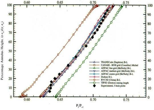
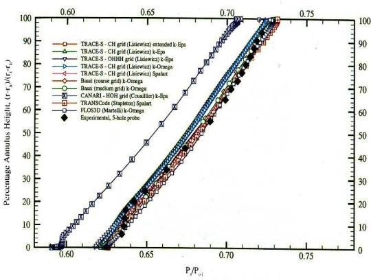
Figure 7: and Figure 8: show the radial distribution of the static pressure ratio in the measuring plane. The slope predicted by the various calculations is in good agreement with the experiments. Differences among the value at fixed radial positions are mainly due to different values of pressure assumed at the reference radius. However, due to the radial equilibrium imposed the small deviation from a linear profile due to the secondary vortices is not recovered in those profiles.
Figure 7: Static Pressure Ratio from algebraic/mixing length models (AGARD-AR-355).
Figure 8: Static Pressure Ratio from turbulent transport models (AGARD-AR-355)
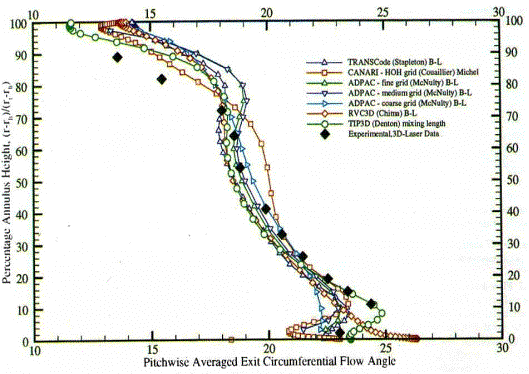
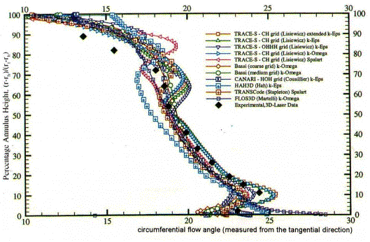
Figure 9: and Figure 10: show the circumferential flow angle profiles from hub to tip produced by codes with both algebraic and transport turbulence models. Since this angle is measured from the tangential direction, it appears that all the flow solvers underestimate the strong overturning in the tip region. Except in this region, some of the codes capture the overturn quite well. This is the case for TRANSCode with both the Baldwin-Lomax and Spalart turbulent models and for TRACE-S code with κ-ε (OHHH and CH grids), extended κ-ε (CH grid), and κ-ω turbulent transport models. For the latter code 117 grid points along the spanwise direction were used. Thus, it seems necessary to use a large number of points in the spanwise direction to obtain a correct representation of the observed circumferential flow angle.
Figure 9: Circumferential Flow angle from algebraic/mixing length models (AGARD-AR-355)
Figure 10: Circumferential Flow angle from turbulent transport models (AGARD-AR-355)
Total pressure ratio on the measuring plane is displayed in Figure 11: and Figure 12:. With the algebraic turbulence models, one can find that all the codes fail to well capture the characteristics of the measurements. Even with the turbulent transport models, no codes were successful in predicting the position and magnitude of loss cores at both the hub and the tip. Models using coarse grids predict a wrong sign of the spanwise gradient. Results are improved when the radial direction is refined. Lisiewicz and Stapleton present two relatively better results with different codes. Lisiewicz applied the TRACE-S code with OHHH grid, κ-ε turbulence model and Stapleton applied the TRANSCode with Spalart turbulence model. Both were using more points in the spanwise direction (117 points for TRACE-S).
Two codes were using the Spalart turbulence closure model. Whereas the results from TRANSCode do well reproduce the experimental data, the results from TRACE-S with the same turbulence model experiments a wrong pressure gradient in the core flow. Such a difference reflect the fact that the Spalart model was not "mature" enough in the early 90's and that the result from the TRACE-S code with this model is not representative of the present state of the art.
Figure 11: Total Pressure Ratio from algebraic/mixing length models (AGARD-AR-355).
Figure 12: Total Pressure Ratio from turbulent transport models (AGARD-AR-355).
Two examples of the total pressure ratio distribution on the measuring plane are displayed on Figure 13: (for comparison experimental data could be found in Figure 24:). All the models exhibit a more or less pronounced "S" – shaped distortion of the wake. The better results are obtained with the TRACE-S code (performed with the greatest number of points in the spanwise direction). From those results it appears that the turbulence model influences the mean total pressure field less than the grid radial spacing.
Figure 13: Total Pressure Ratio (a)Bassi using k-ω turbulence model (b) TRACE-S code using k-ε model (AGARD-AR-355)
Mach number on the measuring planes is shown in Figure 14: and Figure 15:. These graphs are only a combination of the pressure and total pressure ones, and their general trend is satisfactory. However, algebraic/mixing length turbulence models fail to predict the local minimum Mach number close to the hub (at approximately 15 % in the spanwise direction), whereas most of the turbulent transport models do reproduce this pattern. From 70 to 80 % of the spanwise distance, most of the codes using a turbulent transport model exhibit a change in the Mach number gradient from hub to tip. Whereas 3D-laser data are almost linear in this region, a small change in the sign of the gradient could be identified from 5-hole probe measurements. Figure 16:shows the measurement for the Mach number in the downstream plane with the two different measuring techniques. From this figure it is clear that 5-hole probe do better capture the fine structures of this 2D profile than 3D-laser data.
Figure 14: Mach Number from algebraic/mixing length models (AGARD-AR-355)
Figure 15: Mach Number from turbulent transport models (AGARD-AR-355)
Figure 16: Mach Number Measurement (a) Five Hole Probe (b) 3D Two Focus
Two examples of the viscosity ratio distribution on the measuring plane are displayed on Figure 17:. This illustrates the "surprising" huge scatter in the predicted viscosity ratio resulting from all the computations performed in the AGARD study. A difference of more than one order of magnitude in this field has even been observed for the same code using two different turbulent transport models. Such a scatter was attributed to differences in the practical implementation of the turbulence models, and not to the physical and mathematical aspects of these models.
Figure 17: Viscosity Ratio (a) Bassi using k-ω (b) Lisiewicz using k-ω
The main conclusions of this report were:
- The number of cells in the spanwise direction is of great importance. This is particularly true inside the main flow where the refinement of the mesh is often neglected in favor of the boundary layer region.
- The global features are much better solved than the local features; especially in the near end-wall regions where the 3D effects induced by the secondary flows are significant. A mesh of the order of 500,000 adequately distributed points, is said to be sufficient to get a good simulation of annular turbine stators.
- The turbulence modeling is said not to be the principal source of discrepancy for this type of simulation. Acceptable solutions can be obtained with a large scatter in the prediction of the turbulence quantities. However, two-equation transport models did have a tendency to better prediction, compared to algebraic/mixing length models. Furthermore, this analysis has not examined the mixing process and the heat transfer at the wall. The turbulence modeling could then become of much higher importance.
New calculations
The mass flow rates and the total pressure coefficients calculated with different turbulence models and grids are shown in the following table for the ten new calculations performed with the FINE EURANUS/Turbo flow solver.
|
|
|
Turbulence Model |
Total pressure coefficient |
|
| |
|
|
| |||||
|
|
|
Baldwin-Lomax |
|
|
|
|
|
|
Low Re Chien |
|
|
|
| |
|
|
|
|
|
| ||
|
|
Low Re Yang-Shih |
|
|
|
| |
|
|
|
|
|
| ||
|
|
Low Re Launder-Sharma |
|
|
|
| |
|
|
Standard κ-ε Wall function |
|
|
|
| |
|
|
|
|
|
| ||
|
|
0.6-0.7 |
Low Re Chien |
|
|
|
|
|
|
Low Re Yang-Shih |
|
|
|
| |
|
|
|
|
|
|
| |
For some of the turbulence models two results are provided. They correspond to two different values of the inlet turbulent dissipation.
The total pressure coefficient is defined as (P02-P2)/(P01-P2).
The mass flow rates of all the computations remain more or less the same, the error of the calculated mass flow compared with the experimental is among 1.1% to 1.9%
From this table one can draw two conclusions:
- The inlet turbulence dissipation does not influence the global performance.
- The y+ has an obvious influence on the global performance. The computations with two grids are both carried out with the Low Reynolds Yang-Shih and Chien turbulence models. The total pressure coefficient is changed from 0.9 to 0.92 for the Low Reynolds Chien model and 0.89 to 0.92 for the Low Reynolds Yang-Shih model.
The comparison with the experiment is performed on the downstream measurement plane. The results of different turbulence models with the y+ of 6 and inlet turbulent dissipation being 232000 m2/s3 are selected to compare with the experiment.
Figure 18: shows the radial distribution of the static pressure ratio. Since the averaged experimental static pressure at midspan was imposed at the outlet boundary and the simple radial equilibrium method was used, the static pressure distributions along the spanwise direction of all the turbulence models are almost identical and agree with the experiment. However, are previously noticed for the AGARD study, small deviation from a linear profile due to the secondary vortices is not recovered in those profiles.
Figure 18: Static Pressure Ratio
Figure 19: shows the circumferential angle profile from hub to tip in the measuring plane. The different turbulence models captured the overturn of the flow both in the tip and hub area. A difference of 1 to 2 degree is observed. The flow overturn is better captured near the hub than near the shroud, both in location and size. As for the AGARD study, the overturning is under-estimated in the tip region. A possible explanation is that the secondary flow and the two legs of the horseshoe vortex are stronger near the tip than near the hub. Also, since the measuring plane is much closer to the trailing edge near the tip, the wake effect is higher. In this case, more grid points should be used in the spanwise direction, especially near the tip.
Figure 19: Circumferential flow angle
Figure 20:, Figure 21:, and Figure 22: show the 5-hole probe measured and calculated circumferential flow angles with different turbulence models. Good agreement can be found between the measured and numerical results. Little differences can be found with the magnitude of the flow overturn in the tip and hub loss core. The maximum flow angle of the measurement at the tip and hub is 22.0 and 30.0 degree respectively, which is about 2 and 4 degrees larger than the simulation results.
Figure 20: Circumferential Flow Angle (a) Measurement (b) Baldwin-Lomax
Figure 21: Circumferential Flow Angle (a) Low Reynolds Chien (b) Low Reynolds Launder Sharma
Figure 22: Circumferential Flow Angle (a) Standard (b) Low Reynolds Yang-Shi
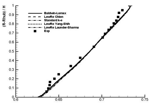
Figure 23: shows the total pressure ratio profile from hub to tip in the measurement plane. All the turbulence models display good agreements with the experiment. The significant features of the measurements are captured fairly well. Two loss cores are identified, that corresponds to the location of the center of the passage vortices. The near-hub loss core is located at about 11% of the blade height away from the hub and the near shroud one is located at about 55% away from the hub. These are both well captured by the numerical results. Nonetheless, the loss core at the hub is better captured than the one at the tip. The under-estimation of the latter loss core is linked to the under-estimation of the overturning in this region.
Divergences of the total pressure ratio in the tip and hub loss core area can be found for different turbulent transport models. In this case, it is hard to tell which turbulence model is the best, because, as can be seen in Figure 23:, the Low Reynolds Chien model matches the experimental data better in the near loss core area of the hub, while the standard κ-ε plus wall function model matches the experimental data better in the near loss core area of the tip.
One impressive thing is that the result of the Baldwin-Lomax turbulence model is fairly good compared with the two equations turbulence models. Thus one can draw the conclusion that in the subsonic flow with no obvious separation, two equations turbulent transport models do not show their advantages in simulating the flow field. Hence, the Baldwin-Lomax algebraic turbulence model should be preferred due to its good convergence and easier implementation.
Another interesting thing is the difference between the Low Reynolds Yang-Shih model and the standard κ-ε plus wall function model. Indeed, the wall function method is developed directly from the Low Reynolds Yang-Shih model, with adaptation at the near wall field. However, obvious difference of the total pressure ratio distribution can be found between the two models throughout the span. The possible reason is the difference of the best-working range of y+ for the two models. For the Low Reynolds Yang-Shih model, the preferable value for y+ is under 1, while for the wall function model, the y+ can be changed in a wide range of value. Hence, the value of 6 for y+ may cause the difference between the two turbulence models.
Figure 23: Total Pressure ratio
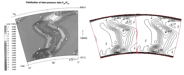
The total pressure ratio distribution is shown on Figure 24:, Figure 25:, and Figure 26:. All calculated results with various turbulence models agree with the experiment very well. They all clearly display the distortion of the wake and two loss cores at hub and tip can be found. The measured loss cores at hub and tip are located at about 12% and 55% of the blade height away from hub.
One can see that the algebraic Baldwin-Lomax model behaves very well when compared with the turbulence transport models. The Baldwin-Lomax shifts the loss core of the tip to about 5% higher than the experiment, while the Low Reynolds Launder-Sharma shifts the tip loss core about 5% lower than the experiment. The standard k-ε plus wall function, Low Reynolds Chien and Yang-Shih models predict the tip loss core approximately at the correct location. The total pressure ratio gradient of Low Reynolds Chien model is higher than other models, which in some sense means the wake is less developed. The differences between these turbulence models are possibly caused by the differences in the boundary layer development, either the boundary layer thickness or the different velocity profiles in the boundary layer. With different boundary layer development, the mixing of the horseshoe vortex, passage vortex and the wake can result in a slightly different position and magnitude of the loss in the wake.
Figure 24: Total Pressure Ratio (a) Measurement (b) Baldwin-Lomax
Figure 25: Total Pressure Ratio (a) Low Reynolds Chien (b) Low Reynolds Launder-Sharma
Figure 26: Total Pressure Ratio (a) Standard (b) Low Reynolds Yang-Shih
Figure 27: shows the radial distribution of the Mach number at the measurement plane. Computations do reproduce the local maximum in the hub region and a change in the sign of the Mach number gradient at about 70 % of the spanwise distance (only visible in the 5-hole probe data).
Figure 27: Mach Number
Figure 28:, Figure 29:, and Figure 30: show the computed Mach number obtained with the different turbulence models (experimental data are provided on Figure 16:). All the models are able to capture the structure of the Mach number distribution on the measuring plane and difference between models are rather small.
Figure 28: Mach Number (a) Baldwin-Lomax (b) Low Reynolds Chien
Figure 29: Mach Number (a) Low Reynolds Launder Sharma (b) Standard
Figure 30: Mach Number from Low Reynolds Yang-Shi.
Figure 31: and Figure 32:show the ratio between the laminar and the turbulent viscosity for the four turbulent transport models. This quantity allows identifying the wake area and the two local maxima in the passage vortex. Contrary to what has been observed in the AGARD study, all models give similar results. The low Reynolds Launder-Sharma and Yang-Shih model show stronger gradient and capture strong turbulent flow in the wake area.
Figure 31: Viscosity Ratio (a) Low Reynolds Chien (b) Low Reynolds Launder-Sharma
Figure 32: Viscosity Ratio (a) Standard (b) Low Reynolds Yang-Shi
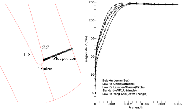
Figure 33: shows the velocity profile at midspan of the suction surface near the trailing edge. The velocity magnitudes in the mainstream of all the turbulence models keep the same value, while the boundary thickness and velocity profile in the boundary layer differ. Therefore, even if 2D-structures are similar in the measuring plane and are closed to observations, differences could be identified in the velocity profiles near the blade surface.
Figure 33: Velocity in the Boundary Layer at midspan
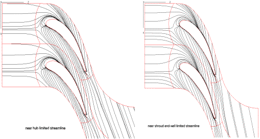
Though a detail description of the simulated 3D flow could be found out of the scope of the present UFR, it seems necessary to perform such a brief description in order to better understand all the phenomenon occurring in this turbine cascade. Figure 34: shows the limit streamlines on hub and shroud. At the design point, the limit streamlines are not strongly turned by the pressure gradient between the pressure and suction side, which means the passage vortex is not very strong. The horseshoe vortex is significant because the leading edge is relatively thick. The suction leg of the horseshoe vortex is pushed by the pressure gradient to the suction surface at about 30% of the axial chord and the pressure leg of the horseshoe vortex develops to about 35% of the axial chord and then hit the suction side, which means the pressure and suction leg vortices will go across each other when they develop downstream.
Figure 34: Limit Streamlines at End Walls
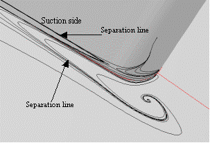
Small separations can be found at the trailing edge of both the near hub and shroud regions, as shown in Figure 35:.
Figure 35: Separation at the Trailing Edge
Figure 36: shows the limit streamline of the blade surfaces. Separation lines can be seen clearly at the suction side. They correspond to the passage vortex. The tip passage vortex is much stronger than the hub one.
Figure 36: Limit Streamlines on Blade Surfaces
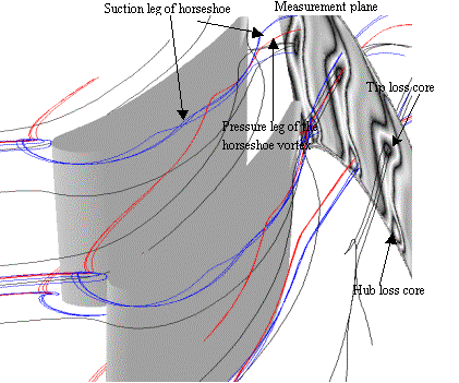
Figure 37: shows the horseshoe vortices with volume streamlines. The suction leg of the horseshoe vortex rotates clockwise and is pushed forward by the transverse pressure gradient. It rotates in the opposite direction compared to the passage vortex. On the contrary, the pressure leg of the horseshoe vortex rotates counterclockwise and has the same rotation direction as the passage vortex. Thus it rotates stronger than the suction leg. The two legs cross each other as they develop downstream near the tip and mix with the wake. They also mix with the passage vortex into the loss core of the tip as it is shown at the measurement plane. The same thing happens to the horseshoe vortex near the hub.
Figure 37: Horse Vortices Visualisation
The passage vortex is not very strong because there is not a high turning of the profile. Thus the stream near the tip rotates only about one and a half rounds when it passes through from the inlet to the exit.
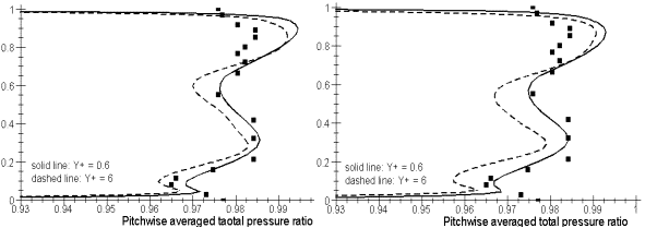
In Figure 38:, results of the Chien and Yang-Shih models are presented. The dashed lines are the results with y+=6, the solid lines are those with y+=0.6, while the experimental results are displayed with solid squares. The difference is significant. Both turbulence models captured the hub and tip loss cores better with smaller y+. Since the different vortices are initiated by the end wall boundary layers and the wake is generated by the boundary layers on the blade, a better resolution of the flow in the boundary layer will result in a better result of capturing the loss where vortices and wake mix. With the y+ being 0.6, more grids are placed in the boundary area, which is necessary for the simulation of viscous flow.
Figure 38: Influence of y+ on Total Pressure Ratio (a) Chien (b) Yang-Shih models
The major conclusions that can be inferred from these simulations are:
- The algebraic model of Baldwin-Lomax is good enough for this kind of flow. The global performance is indeed fairly well predicted with this model and the more detailed aspects of the flow are reasonably well predicted. Owing to its relatively low cost in memory and CPU time, this model should be found appropriate for this type of flow regime.
- It has been shown that a critical factor of the precision is a good grid resolution of the boundary layers. These give birth to the loss mechanisms of this UFR. It is therefore important to use a clustering to the solid walls corresponding to a y+ of 1 or less and to place enough points in the whole boundary layer thickness.
- The low Reynolds Yang-Shih model appears more sensitive to y+ than the low Reynolds Chien model.
- The most pronounced difference between the four k-ε turbulence models lies in the total pressure ratio at the measuring plane. The total pressure ratio gradient of the low Reynolds Chien model is higher than for the other models.
© copyright ERCOFTAC 2004
Contributors: Nouredine Hakimi - NUMECA International
