UFR 3-09 Evaluation: Difference between revisions
m (UFR 3-09 Evaluation moved to Gold:UFR 3-09 Evaluation) |
|||
| Line 37: | Line 37: | ||
Craft, T. J. & Launder, B. E. 1996. A Reynolds stress closure designed for complex geometries. Int. J. Heat and Fluid Flow 17, 245-254. | Craft, T. J. & Launder, B. E. 1996. A Reynolds stress closure designed for complex geometries. Int. J. Heat and Fluid Flow 17, 245-254. | ||
Another approach to impose the selective damping of the wall-normal fluctuations is applied in computation t. The method used to reproduce the blocking effect of the wall is derived from Durbin's elliptic relaxation method. However, the Elliptic Blending Model (EBM) uses a single blending function, which satisfies an elliptic relaxation equation, instead of 6 functions, from 6 equations, in Durbin's original model. Contrary to the cubic model of computation d, the EBM is based on a linear pressure strain model. This thus a very promising, simple way of reproducing the blocking effect of the wall. Note that the model is very recent (Manceau & Hanjalic, and has not reached a definitive, well calibrated form yet. | Another approach to impose the selective damping of the wall-normal fluctuations is applied in computation t. The method used to reproduce the blocking effect of the wall is derived from Durbin's elliptic relaxation method. However, the Elliptic Blending Model (EBM) uses a single blending function, which satisfies an elliptic relaxation equation, instead of 6 functions, from 6 equations, in Durbin's original model. Contrary to the cubic model of computation d, the EBM is based on a linear pressure strain model. This thus a very promising, simple way of reproducing the blocking effect of the wall. Note that the model is very recent (Manceau & Hanjalic), and has not reached a definitive, well calibrated form yet. | ||
Manceau, R. & Hanjalic, K. 2002. Elliptic Blending Model: A New Near-Wall Reynolds-Stress Turbulence Closure. Phys. Fluids 14, 744-754. | Manceau, R. & Hanjalic, K. 2002. Elliptic Blending Model: A New Near-Wall Reynolds-Stress Turbulence Closure. Phys. Fluids 14, 744-754. | ||
| Line 51: | Line 51: | ||
|} | |} | ||
<br clear="ALL" /> | <br clear="ALL" /> | ||
<br clear="ALL" /> | <br clear="ALL" /> | ||
| Line 65: | Line 65: | ||
|} | |} | ||
<br clear="ALL" /> | <br clear="ALL" /> | ||
<br clear="ALL" /> | <br clear="ALL" /> | ||
| Line 79: | Line 79: | ||
|} | |} | ||
<br clear="ALL" /> | <br clear="ALL" /> | ||
<br clear="ALL" /> | <br clear="ALL" /> | ||
| Line 93: | Line 93: | ||
|} | |} | ||
<br clear="ALL" /> | <br clear="ALL" /> | ||
<br clear="ALL" /> | <br clear="ALL" /> | ||
| Line 107: | Line 107: | ||
|} | |} | ||
<br clear="ALL" /> | <br clear="ALL" /> | ||
<br clear="ALL" /> | <br clear="ALL" /> | ||
| Line 121: | Line 121: | ||
|} | |} | ||
<br clear="ALL" /> | <br clear="ALL" /> | ||
<br clear="ALL" /> | <br clear="ALL" /> | ||
| Line 135: | Line 135: | ||
|} | |} | ||
<br clear="ALL" /> | <br clear="ALL" /> | ||
<br clear="ALL" /> | <br clear="ALL" /> | ||
| Line 149: | Line 149: | ||
|} | |} | ||
<br clear="ALL" /> | <br clear="ALL" /> | ||
<br clear="ALL" /> | <br clear="ALL" /> | ||
| Line 163: | Line 163: | ||
|} | |} | ||
<br clear="ALL" /> | <br clear="ALL" /> | ||
<br clear="ALL" /> | <br clear="ALL" /> | ||
| Line 177: | Line 177: | ||
|} | |} | ||
<br clear="ALL" /> | <br clear="ALL" /> | ||
<br clear="ALL" /> | <br clear="ALL" /> | ||
| Line 191: | Line 191: | ||
|} | |} | ||
<br clear="ALL" /> | <br clear="ALL" /> | ||
<br clear="ALL" /> | <br clear="ALL" /> | ||
| Line 205: | Line 205: | ||
|} | |} | ||
<br clear="ALL" /> | <br clear="ALL" /> | ||
<br clear="ALL" /> | <br clear="ALL" /> | ||
| Line 219: | Line 219: | ||
|} | |} | ||
<br clear="ALL" /> | <br clear="ALL" /> | ||
<br clear="ALL" /> | <br clear="ALL" /> | ||
| Line 233: | Line 233: | ||
|} | |} | ||
<br clear="ALL" /> | <br clear="ALL" /> | ||
<br clear="ALL" /> | <br clear="ALL" /> | ||
| Line 247: | Line 247: | ||
|} | |} | ||
<br clear="ALL" /> | <br clear="ALL" /> | ||
<br clear="ALL" /> | <br clear="ALL" /> | ||
| Line 261: | Line 261: | ||
|} | |} | ||
<br clear="ALL" /> | <br clear="ALL" /> | ||
<br clear="ALL" /> | <br clear="ALL" /> | ||
| Line 275: | Line 275: | ||
|} | |} | ||
<br clear="ALL" /> | <br clear="ALL" /> | ||
<br clear="ALL" /> | <br clear="ALL" /> | ||
| Line 289: | Line 289: | ||
|} | |} | ||
<br clear="ALL" /> | <br clear="ALL" /> | ||
<br clear="ALL" /> | <br clear="ALL" /> | ||
| Line 303: | Line 303: | ||
|} | |} | ||
<br clear="ALL" /> | <br clear="ALL" /> | ||
<br clear="ALL" /> | <br clear="ALL" /> | ||
| Line 317: | Line 317: | ||
|} | |} | ||
<br clear="ALL" /> | <br clear="ALL" /> | ||
<br clear="ALL" /> | <br clear="ALL" /> | ||
Revision as of 09:45, 12 May 2009
Impinging jet
Underlying Flow Regime 3-09 © copyright ERCOFTAC 2004
Evaluation
Comparison of CFD calculations with Experiments
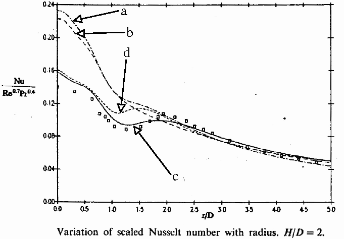
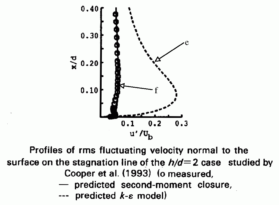
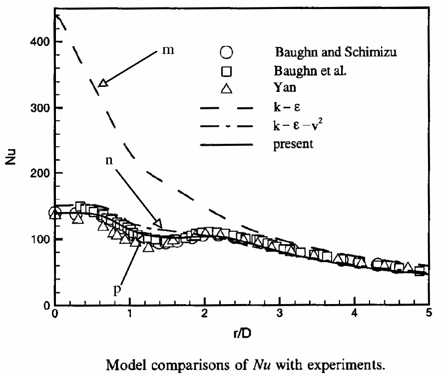
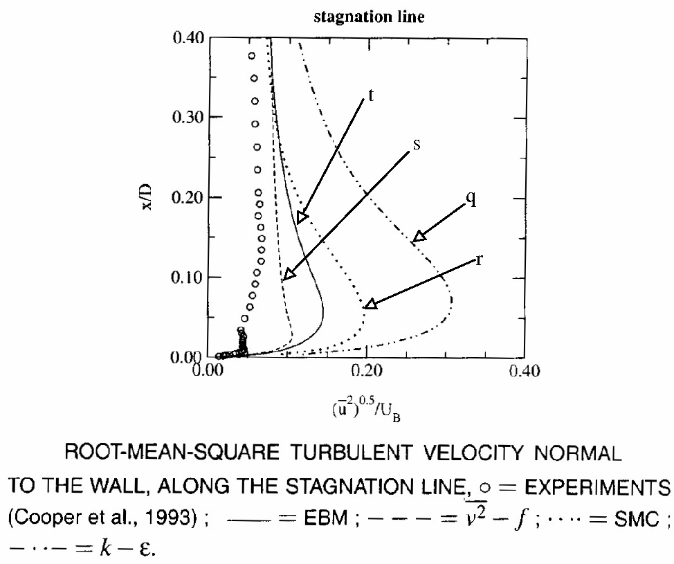
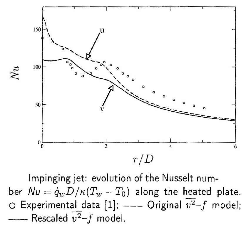
The first striking point when going through all the results is the fact that the prediction of the Nusselt number distribution is highly dependent on the prediction of the turbulence in the vicinity of the impingement point, and in particular on the prediction of the Reynolds stresses involving fluctuations normal to the wall (uv and vv) which mainly drive the diffusion processes from and toward the wall. For instance, it can be seen in Fig. 2 and Fig. 3, that the two models (computation a and b) which does not predict correctly the wall-normal fluctuation (attention must be drawn to the fact that some authors call it u', some others v') are also unable to predict the Nusselt number in the impingement region. This is confirmed by Fig. 18 and Fig. 19, in which the strong overestimation of the wall-normal fluctuation by computation q (k-epsilon model) yields a similar strong overestimation of the Nusselt number. This is also confirmed by other studies using k-epsilon models (computations k and m), for which the Nusselt number is overpredicted by a factor of 2.5, at least (see Fig. 9 and Fig. 15). The comparison between computations a and b (Fig. 3) yields another conclusion: the well-known overestimation of turbulent energy in plane strain situations (due to the fact that the production term in the k-epsilon model is quadratic in the strain rate) is not the main issue in this case, since the second-moment closure gives the same overestimation. It plays in the wrong direction, but is overweighted by the absence of reproduction of the damping of wall-normal diffusion. However, it is worth pointing out that eddy-viscosity models reproducing the wall damping correctly (computations l, n, p, s, u, v, x) are also not affected by the overestimation-of-production problem since they involve time-scale limiters (computations l, n, s, u, v, x) or their eddy-viscosity derives from a second-moment closure (computation p).
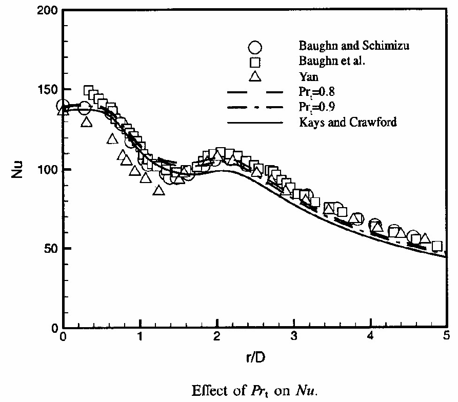
Most of the studies indicate that the turbulent fluxes model does not play a primary role. First, Park & Sung showed, as can be seen in figure Fig. 14, that the Nusselt number prediction is not very sensitive to a change in the turbulent Prandtl number model used in the turbulent diffusivity model (computation p). Moreover, Fig. 3 is very interesting from this point of view: firstly, computations a and b use very different models for the turbulent heat fluxes (a: eddy diffusivity; b: Transport model), and they give very similar, wrong Nusselt number predictions, which indicates that this prediction is much more sensitive to the spurious prediction of the turbulent field than to the refinement of the model for the turbulent heat fluxes (however, it is worth pointing out that the same Launder-Sharma/turbulent diffusivity model is used in the near-wall region for all the computations made by Craft et al.); secondly, computations c and d, both predicting the turbulent field correctly, give very similar, satisfactory Nusselt number distributions, despite the fact that computation d uses a more refined model for the turbulent heat fluxes. The present observation is further sustained by Fig. 4: the inclusion of the Yap correction in the epsilon equation, which only influences the turbulent field very close to the wall, has a huge effect on the Nusselt number prediction in the impingement region. Simarly, by using wall functions which can be used with very fine meshes (scalable wall functions), the results of the k-epsilon model are improved, by artificially constraining the turbulent scales in the viscous sublayer (computation w, Fig. 23).
However, this strict dependence on the turbulence model is a consequence of the fact that the turbulent heat fluxes are more or less directly linked to the Reynolds stresses in the models used in the studies quoted above. With the q-dzeta turbulence model (computation h and i), the prediction of the turbulence field is probably not very good (very few details given in the paper), such that the Nusselt number as predicted by computation h is far too high. However, changing the turbulent heat fluxes model from a simple eddy diffusivity model with a constant Prandtl number to a two equation model, with a correct asymptotic damping of the heat fluxes at the wall, leads to a much better Nusselt number prediction. This reveals a simple mechanism: deficiencies of the turbulence model (absence of damping of the wall-normal momentum transport) yield wrong predictions of the turbulent heat fluxes when the model for the latter is directly linked to the former: introducing proper damping of the turbulent heat fluxes in the near-wall region (computation i) helps correcting the problem; on the contrary, when the turbulence model gives a satisfactory near-wall turbulence field, all the models for the turbulent heat fluxes, even very simple, lead to good predictions of the Nusselt number distribution.
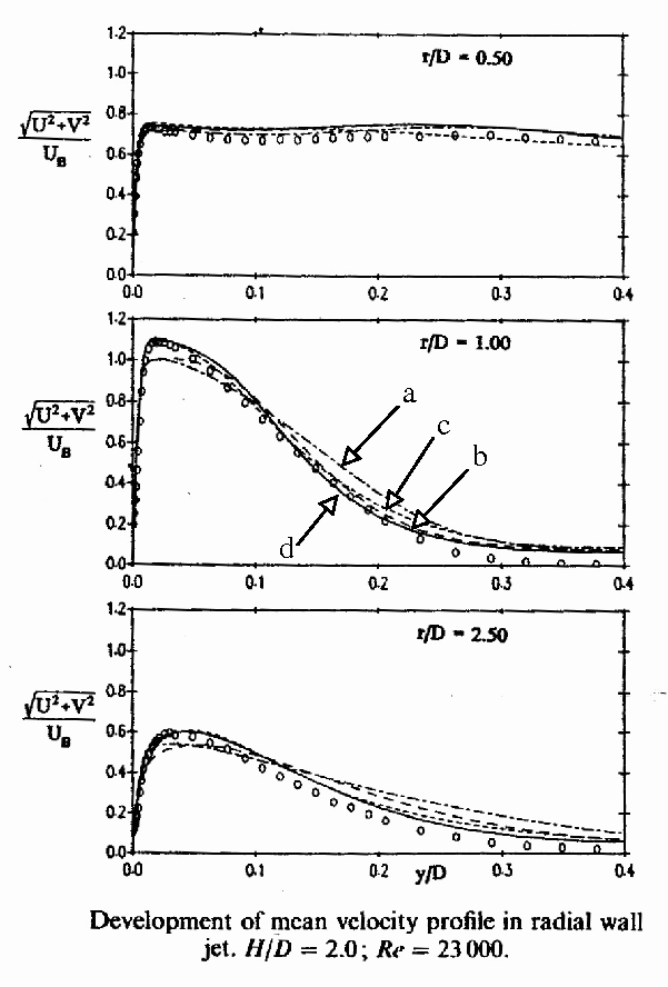
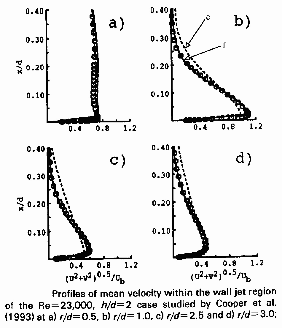
A strong influence of the turbulent field is also observed on the development of the radial wall jet. All the computations (a, b, e, g, h, k, m and q, w) using models which overestimate the turbulent fluctuations exhibit a wrong development of the wall jet, with an underestimation of the mean velocity below x/D=0.1 and an overestimation above (see Fig. 1, Fig. 5, Fig. 7, Fig. 13, Fig. 16, Fig. 22).
A simple conclusion emerges from all the computations: predicting a correct turbulent field in the impingement region is of primary importance. In particular, the strong damping of the Reynolds stresses involving wall-normal fluctuations (uv and vv) must be correctly predicted, since it drives the turbulent diffusion mechanisms (momentum and heat) between the flow and the wall.
The standard k-epsilon model (computations e, m and q, w) does not contain damping processes at all: the Boussinesq equation states that the Reynolds-stress anisotropies are directly proportional to the corresponding component of the strain tensor. Moreover, the model refers to flows parallel to the wall for their boundary conditions (wall functions). This has mainly too consequences: firstly, the absence of damping of the wall-normal fluctuations leads to an overestimation of the wall-normal diffusion processes; secondly, a simple analysis shows that the eddy viscosity hypothesis implies that high levels of wall-normal Reynolds stress yields high levels of production of turbulent energy in plane strain situations (impingement region), which, in turn, leads to high levels of wall-normal fluctuations. In order to reduce diffusion, low-Reynolds number k-epsilon models, such as the Launder-Sharma model used in computations a, g and k, use damping functions for the eddy-viscosity, without introducing further sensitivity to the presence of the wall than a global damping of all the fluctuations. Thus, this model family yields a severe overestimation of the turbulent fluctuations in the wall-normal direction, leading to much too high levels of the Nusselt number in the impingement region. The same problems occur with the q-dzeta model (see Fig. 5 and Fig. 6), which is basically a standard k-epsilon model written with other variables. The inclusion of the Yap correction in the destruction rate equation of these models (k-epsilon and q-dzeta) improves the results, but is only a patch devised for reducing the diffusion in the impingement region by constraining the turbulent length scale to its equilibrium value.
Standard Reynolds stress models (RSM), such as Gibson-Launder's (computation b), use wall echo terms to impose a damping of the wall-normal fluctuations. However, these terms are calibrated in shear flows. They are derived in order to inhibit the redistribution of energy from the wall parallel to the wall-normal component, but are ill-behaved in impinging flows: the wall-normal fluctuation is actually amplified by the rapid part of the wall echo term, which yields a strong overestimation of this component, and, in turn, of the overall diffusion (see Fig. 2 and Fig. 3). Therefore, Craft et al. and Dianat et al. used new wall echo terms which do not exhibit the same spurious behaviour (computations c and f): the results are then drastically improved (see Fig. 2, Fig. 3 and Fig. 12).
The best way to reproduce the diffusion mechanisms is thus to use a Reynolds stress model with a selective damping of the wall-normal fluctuations. The simplest solution is the use of wall echo terms formulated such that they behave correctly in impinging flows (computations c and f). However, these models cannot be integrated down to the plate and require the use of a k-epsilon model in the near-wall region (computation c) or of wall functions (computation f), which impairs the predictions in the near-wall region. Moreover, the wall-echo terms refer to the concept of "closest wall" and "wall-normal direction" which are often not well defined in complex geometries.
Therefore, different approaches have been developed. In order to reproduce the two-component limit of turbulence, i.e., the strong damping of the wall-normal fluctuations, UMIST team has developed a series of nonlinear formulations of the pressure-strain term. In computation d, a cubic formulation is used, but coupled in the near-wall region with a k-epsilon model. In more recent work of this research team, cubic formulations are integrated down to solid boundaries.
Craft, T. J. & Launder, B. E. 1996. A Reynolds stress closure designed for complex geometries. Int. J. Heat and Fluid Flow 17, 245-254.
Another approach to impose the selective damping of the wall-normal fluctuations is applied in computation t. The method used to reproduce the blocking effect of the wall is derived from Durbin's elliptic relaxation method. However, the Elliptic Blending Model (EBM) uses a single blending function, which satisfies an elliptic relaxation equation, instead of 6 functions, from 6 equations, in Durbin's original model. Contrary to the cubic model of computation d, the EBM is based on a linear pressure strain model. This thus a very promising, simple way of reproducing the blocking effect of the wall. Note that the model is very recent (Manceau & Hanjalic), and has not reached a definitive, well calibrated form yet.
Manceau, R. & Hanjalic, K. 2002. Elliptic Blending Model: A New Near-Wall Reynolds-Stress Turbulence Closure. Phys. Fluids 14, 744-754.
However, even though Reynolds stress models yield in general better predictions of the turbulent field, and in particular of the anisotropies, they increase the complexity of the computation and in particular the number of equations compared to eddy viscosity models. Therefore, for some industrial application, in particular when the quantity of interest is only the Nusselt number, eddy viscosity models can be preferred. In this case, models which reproduce the blocking effect of the wall on the eddy-viscosity are necessary for impinging jets. Three models in the computations described above fulfil this requirement and give very satisfactory results: the V2F model (computations l, n, s, u and v), the k-epsilon-fmu model (computation p) and the SST model (computation x). The first one is now very well known and is related via a theoretical analysis to the true blocking mechanism; the second one uses a more artificial way of blocking the wall-normal fluctuations, but uses a non-equilibrium formulation of the eddy viscosity based on an algebraic form of a Reynolds stress model and, thus, contains more physics than the V2F model; the third one reproduces the damping of the eddy-viscosity through the wall boundary condition of the variable omega. Note that there is an ambiguity in the definition of the wall-normal fluctuation in the case of the V2F model: if it is reconstructed by the Boussinesq equation, it appears to be overestimated (see Fig. 17). However, what enters the eddy-viscosity in is the variable called v2, given by the transport equation: it can be considered the wall-normal fluctuation only close to the wall, but when this definition is used, the wall-normal fluctuation is correctly reproduced (see Fig. 8).
Figure 1, reprinted from the International Journal of Heat and Mass Transfer, Vol. 36 (10), T.J. Craft et al, Impinging jet studies for turbulence model assessment - ii. an examination of the performance of four turbulence models, p. 2685, 1993, with permission from Elsevier.
Figure 2, reprinted from the International Journal of Heat and Mass Transfer, Vol. 36 (10), T.J. Craft et al, Impinging jet studies for turbulence model assessment - ii. an examination of the performance of four turbulence models, p. 2685, 1993, with permission from Elsevier.
Figure 3, reprinted from the International Journal of Heat and Mass Transfer, Vol. 36 (10), T.J. Craft et al, Impinging jet studies for turbulence model assessment - ii. an examination of the performance of four turbulence models, p. 2685, 1993, with permission from Elsevier.
Figure 4, reprinted from the International Journal of Heat and Mass Transfer, Vol. 36 (10), T.J. Craft et al, Impinging jet studies for turbulence model assessment - ii. an examination of the performance of four turbulence models, p. 2685, 1993, with permission from Elsevier.
Figure 5, reprinted from the International Journal of Heat and Fluid Flow, Vol. 18, M.M. Gibson et al, Calculation of impinging-jet heat transfer with the low-reynolds-number q-turbulence model, p. 80, 1997, with permission from Elsevier.
Figure 6, reprinted from the International Journal of Heat and Fluid Flow, Vol. 18, M.M. Gibson et al, Calculation of impinging-jet heat transfer with the low-reynolds-number q-turbulence model, p. 80, 1997, with permission from Elsevier.
Figure 7, reprinted from the International Journal of Heat and Mass Transfer, Vol. 41(12), M. Behnia et al, Prediction of heat transfer in a jet impinging on a flat plate, p. 1845, 1998, with permission from Elsevier.
Figure 8, reprinted from the International Journal of Heat and Mass Transfer, Vol. 41(12), M. Behnia et al, Prediction of heat transfer in a jet impinging on a flat plate, p. 1845, 1998, with permission from Elsevier.
Figure 9, reprinted from the International Journal of Heat and Mass Transfer, Vol. 41(12), M. Behnia et al, Prediction of heat transfer in a jet impinging on a flat plate, p. 1845, 1998, with permission from Elsevier.
Figure 10, reprinted from the International Journal of Heat and Fluid Flow, Vol. 17, M.F.M. Dianat et al, Predictions of axisymmetric and two-dimensional impinging turbulent jets, p. 530, 1996, with permission from Elsevier.
Figure 11, reprinted from the International Journal of Heat and Fluid Flow, Vol. 17, M.F.M. Dianat et al, Predictions of axisymmetric and two-dimensional impinging turbulent jets, p. 530, 1996, with permission from Elsevier.
Figure 12, reprinted from the International Journal of Heat and Fluid Flow, Vol. 17, M.F.M. Dianat et al, Predictions of axisymmetric and two-dimensional impinging turbulent jets, p. 530, 1996, with permission from Elsevier.
Figure 13, reprinted from the International Journal of Heat and Fluid Flow, Vol. 22, T.S. Park et al, Development of a near-wall turbulence model and application to jet impingement heat transfer, p. 10, 2001, with permission from Elsevier.
Figure 14, reprinted from the International Journal of Heat and Fluid Flow, Vol. 22, T.S. Park et al, Development of a near-wall turbulence model and application to jet impingement heat transfer, p. 10, 2001, with permission from Elsevier.
Figure 15, reprinted from the International Journal of Heat and Fluid Flow, Vol. 22, T.S. Park et al, Development of a near-wall turbulence model and application to jet impingement heat transfer, p. 10, 2001, with permission from Elsevier.
Figure 17, reprinted from Thielen et al, Turbulence modeling in a single normally impinging jet, Proceedings of the ASME-PVP Conference, Atlanta, USA 2001, Copyright ASME.
Figure 18, reprinted from Thielen et al, Turbulence modeling in a single normally impinging jet, Proceedings of the ASME-PVP Conference, Atlanta, USA 2001, Copyright ASME.
Figure 19, reprinted from Thielen et al, Turbulence modeling in a single normally impinging jet, Proceedings of the ASME-PVP Conference, Atlanta, USA 2001, Copyright ASME.
Figure 20, reprinted from Manceau et al, A rescaled model: first application to separated and impinging flows. In Rodi et al (editors), Proceedings of the 5th International Symposium on Engineering Turbulence Modeling and Measurements, Mallorca, Spain, 2002, with permission from Elsevier.
Figure 21, reprinted from Manceau et al, A rescaled model: first application to separated and impinging flows. In Rodi et al (editors), Proceedings of the 5th International Symposium on Engineering Turbulence Modeling and Measurements, Mallorca, Spain, 2002, with permission from Elsevier.
© copyright ERCOFTAC 2004
Contributors: Remi Manceau - Université de Poitiers
