UFR 4-18 Evaluation

Flow and heat transfer in a pin-fin array

Front Page

Description

Test Case Studies

Evaluation

Best Practice Advice

References

Evaluation

Comparison of CFD Calculations with Experiments

Discuss how well the CFD calculations of the assessment quantities compare with experiment and with one another. Present some key comparisons in the form of tables or graphical plots and, where possible, provide hyperlinks to the appropriate results database. Results with different turbulence models covering as wide a range as possible should be included in the discussion. However, if too many different calculation results are available (e.g. from workshops) do not present all the comparisons here. A selection should be made showing results only for the most typical and practically important models. Comprehensive comparisons can be made available via a link to the associated databases. Finally, draw conclusions on the ability of the models used to simulate the test case flow.

Global comparisons

Pressure loss coefficient

The following table gives the numerical values of the presure loss coefficient in Ames et al. experiment as well as those obtained in the main computations.

Figure ?? shows these values and compare them to existing correlations from the literature:

• Metzger et al. (1982) :

for $Re_{D}<10^{4}$, Failed to parse (syntax error): {\displaystyle f = 0.317 {Re_D}^{−0.132} } , for $Re_{D}>10^{4}$, Failed to parse (syntax error): {\displaystyle f = 1.76 {Re_D}^{−0.318}}

• Jacob (1938) :

$f=(0.25+0.1175/(P/D-1)^{1.08})Re^{-0.16}$

Large Eddy Simulation shows a very good agreement with the correlations and Ames et al. experimental results. The relative error is equal to 1% end 3% for the two Reynolds numbers, respectively. for both computed Reynolds numbers. The EB-RSM shows a very satisfactory pressure loss coefficient at $Re_{D}=10000$ (1% error) but a worse pressure loss coefficient at $Re_{D}=30000$ (10% error). The kω-SST shows globally good results (7% and 6% errors) and the φ-model poorer results with an error of 17% and 12% for the two Reynolds numbers, respectively.

Wall resolved LES is then the best candidate to obtain almost perfect pressure loss coefficients in the present configuration. The EB-RSM five very good results at the lowest Reynolds number but a substantial error is observed at $Re_{D}=30000$. Although the kω-SST exhibits pretty good results, the physics of the present flow is not well captured and one can't rely on this model. The φ-model has to be avoided for the present configuration in order to compute the pressure loss coefficient.

Pressure loss coefficient values for the different computations

	Ames et al. $Re_{D}=3000$	LES3000	Ames et al. $Re_{D}=10000$	LES10000	EBRSM10000	PHI10000	kwSST10000	Ames et al. $Re_{D}=30000$	EBRSM30000	PHI30000	kwSST30000
Value	0.111	0.1076	0.095	0.0939	0.0963	0.0789	0.0883	0.07	0.0771	0.0615	0.0744
Error (%)	-	3	-	1	1	17	7	-	10	12	6

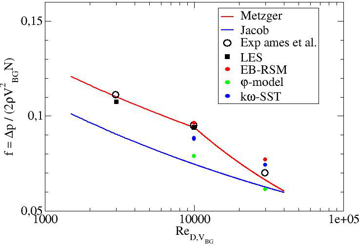
Figure ??: Pressure loss coefficient

Average Nusselt Number

The following table gives the numerical values of the average Nusselt numbers in Ames et al. experiment as well as those obtained in the main computations.

Figure ?? shows these values and compare them to existing correlations from the literature:

• Metzger et al. (1982) :

$Nus=0.079Re^{0.717}$

• Van Fossen (1982) :

$Nus=0.153*Re^{0.686}$

Note that the experimental results have an error of +/- 12%, +/-11.4%, and +/-10.5% for the 3 000, 10 000, and 30 000 Reynolds numbers, respectively, in the endwall regions adjacent to the pins and +/- 9% away from the pin.

One can see that the two models using a first moment closure (φ-model and kω-SST) are too far from the experimental results, except the φ-model at $Re_{D}=30000$ but which, as it will be shown later exhibits a wrong physics. LES and EB-RSM exhibits very satisfactory values in the error interval. The superiority of these two models will be discussed later while dealing with the local normalized Nusselt number on the bottom wall. Ames and Dvorak (2006a) used standard, Realizable and RNG k-ε models in Fluent commercial software. They showed a substantial underestimation of the averaged Nusselt number when the pins were heated. Delibra et al. (2009) used the URANS ζ-f model (very close to the φ-model utilized in the present work) at the 10000 and 30000 Reynolds numbers. They obtained averaged Nusselt numbers of 46.2 and 122.3, respectively. These values are higher than those obtained in the present work and closer to experimental values.The temperature was imposed at the wall in Delibra et al. (2009). Imposing the temperature at the wall in the present work with the φ-model led to averaged Nusselt numbers of 41 and 100, respectively. This shows that imposing the temperature gives higher Nusselt numbers that by imposing the heat flux with this model. The effect of the temperature boundary condition has also been tested with the LES at $Re_{D}=10000$ and the EB-RSM at $Re_{D}=30000$. The averaged Nusselt numbers were equal to 46 and 115.2, respectively. No clear conclusion can be drawn for these two models which give a more realistic physics than the models using a first moment closure concerning the effect of imposing the temperature instead of the heat flux at the bottom wall. However, one can state that there is a difference between the two methods. Delibra et al. (2008) also reported LES computations. The one used for $Re_{D}=30000$ was too coarse with a short time integration and will not be considered here. LES at $Re_{D}=10000$ gave an average Nusselt number equal to 44.3 which is lower than the one obtained in the present work even with a fixed temperature at the wall. The error compared to the experimental value is equal to 18% which is too high. This discrepancy can be attributed to two factors:

• the mesh was probably still too coarse, not in the wall normal directions but in the stream-wise and span-wise ones (the mesh in the present study contains 76 million cells and their mesh contained 5.5 million cells),

• the boundary condition using an imposed temperature is less representative of the experiment.

Finally, Delibra et al. (2010) tried to use a hybrid RANS/LES approach to overcome the understimation of the Nusselt number but the results where close to the ones obtained with the URANS approach based on the ζ-f model.

Average Nusselt number on the bottom wall

	Ames et al. 3000	LES3000	Ames et al. 10000	LES10000	EBRSM10000	PHI10000	kwSST10000	Ames et al. 30000	EBRSM30000	PHI30000	kwSST30000
Value	22.1	21.6	54.1	48.6	48.1	37.6	33.1	111.5	114.8	93.3	72
Error (%)	-	2	-	10	11	30	39	-	3	16	35

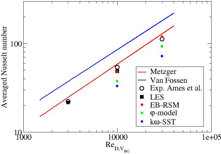
Figure ??: Averaged Nusselt number on the bottom wall

Local comparisons

Mean pressure coefficient

Figures ?? to ?? give the profiles of the pressure coefficient along the midline of pins 1, 2, 3 and 5 for the three Reynolds numbers.

Note that the experimental results have an uncertainty equal to +/-0.075 at $Re_{D}=3000$ and to +/-0.025 at $Re_{D}=10000$ and $Re_{D}=30000$.

LES results are in relatively good agreement with the experimental data. EB-RSM exhibits decent results as well. The two first moment closure models show poor results in particular the φ-model. The prediction of the $C_{p}$ coefficient may be related to the wake prediction downstream the pins.

Figures ?? and ?? display the mean stream-wise velocity field in the midplane (Z=H). The wakes donwstream the cylinders are similar in LES and EB-RSM. The wakes are shorter downstream the cylinders from row 4. The longer wakes are obtained for rows 1 and 2, then then lengths decreases. This is not observed at all for the φ-model and the kω-SST models. One can state at this stage that first moment closures are not able the predict the present flow. One will still plot the values obtained with these two models but without analysing deeply the results.

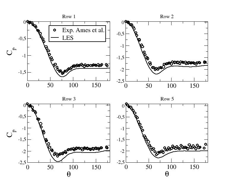
Figure ??: Pressure coefficient along the midline of the pins - LES at $Re_{D}=3000$

Figure ??: Pressure coefficient along the midline of the pins - LES and URANS computations at $Re_{D}=10000$

Figure ??: Pressure coefficient along the midline of the pins - URANS computations at $Re_{D}=30000$

Figure ??: Mean stream-wise velocity in the midplane z=H at $Re_{D}=10000$

Figure ??: Mean stream-wise velocity in the midplane z=H at $Re_{D}=30000$

Mean velocity profiles

Figures ?? show the mean axial velocity line B for the different computations. The first moment closure exhibits a dramatic deficit of the mean axial velocity. On the other hand, LES and EB-RSM perform well compared to the experimental data with a slight overestimation of the mean stream-wise velocity peaks close to the walls in several locations, in particular departin from row 4. Note that the convergence study shown in "Test Case Studies" section proved that the needed refinement to obtain a "convergent" solution around pin 2 is very important (with the first two levels of refinement, a definit in the central velocity was observed).

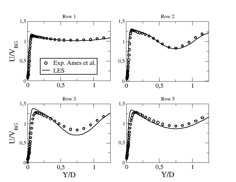
Figure ??: Mean stream-wse velocity component along line B - LES at $Re_{D}=3000$

Figure ??: Mean stream-wse velocity component along line B - LES and URANS computations at $Re_{D}=10000$

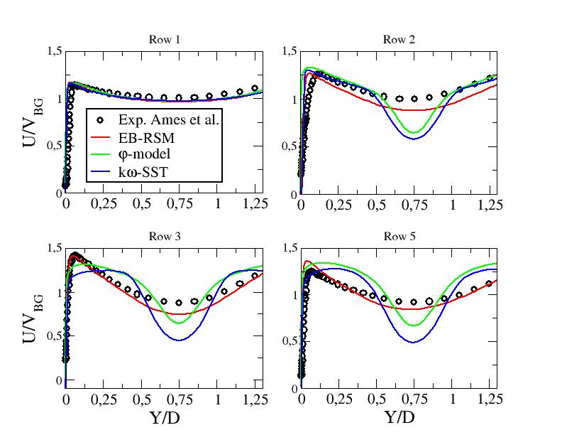
Figure ??: Mean stream-wse velocity component along line B - URANS computations at $Re_{D}=30000$

Figure ??: Mean stream-wse velocity component along line A1 - URANS computations at $Re_{D}=30000$

R.m.s. velocity profiles

Figures ?? show the r.m.s. value of the stream-wise velocity along line B. The first moment closure exhibits behavior which have nothing to do with the experimental measurements (the trends don't correspond at all). On the other hand, LES and EB-RSM perform well compared to the experimental data with a certain superiority of LES. One can notice an overestimation of the r.m.s. value of the stream-wise velocity with the EB-RSM. Figures ?? give the detail of the resolved and modelled stresses for the two Reynolds numbers at which the test case is performed with URANS approaches. One assumes here that $R_{ij}={\overline {u'_{i}u'_{j}}}+{\overline {R}}_{ij}$.

(the whole computational domain is not represented)

Figure ??: R.m.s. of the stream-wise velocity component along line B - LES at $Re_{D}=3000$

Figure ??: R.m.s. of the stream-wise velocity component along line B - LES and URANS computations at $Re_{D}=10000$

Figure ??: Resolved and modelled contributions to the r.m.s. of the stream-wise velocity component along line B - URANS computations at $Re_{D}=10000$

Figure ??: R.m.s. of the stream-wise velocity component along line B - URANS computations at $Re_{D}=30000$

Figure ??: Resolved and modelled contributions to the r.m.s. of the stream-wise velocity component along line B - URANS computations at $Re_{D}=30000$

Figure ??: R.m.s. of the stream-wise velocity component along line A1 - URANS computations at $Re_{D}=30000$

Figure ??: Resolved and modelled contributions to the r.m.s. of the stream-wise velocity component along line A1 - URANS computations at $Re_{D}=30000$

Figure ??: Resolved and modelled contributions to the r.m.s. of the stream-wise velocity component in the midplane - LES and URANS computations at $Re_{D}=10000$

Figure ??: Resolved and modelled contributions to the r.m.s. of the stream-wise velocity component in the midplane - URANS computations at $Re_{D}=30000$

Strouhal numbers

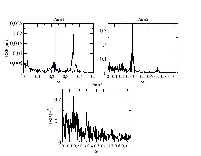
Figure ??: DSP of the stream-wise velocity component at a distance equal to 0.03D normal to the pins and in the mid-plane - Pins 1, 2 and 3 - $Re_{D}=3000$ - black: LES, blue: Ames et al. exp.

Figure ??: DSP of the stream-wise velocity component at a distance equal to 0.03D normal to the pins and in the mid-plane - Pins 1, 2 and 3 - $Re_{D}=10000$ - black: LES, red: EB-RSM, blue: Ames et al. exp.

Figure ??: DSP of the stream-wise velocity component at a distance equal to 0.03D normal to the pins and in the mid-plane - Pins 1, 2 and 3 - $Re_{D}=30000$ - red: EB-RSM, blue: Ames et al. exp.

Nusselt number on the bottom wall

Figure ??: Local Nusselt number on the bottom wall - LES computation at $Re_{D}=3000$ vs. experimental results from Ames et al.

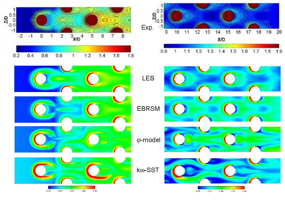
Figure ??: Local Nusselt number on the bottom wall - LES and URANS computations at $Re_{D}=10000$ vs. experimental results from Ames et al.

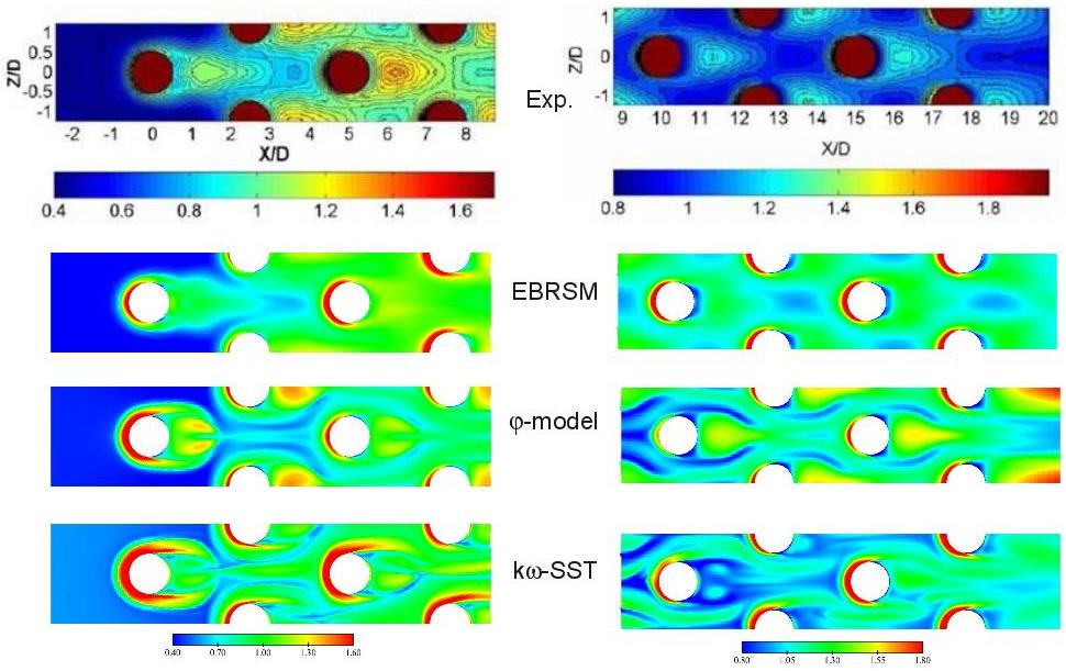
Figure ??: Local Nusselt number on the bottom wall - URANS computations at $Re_{D}=30000$ vs. experimental results from Ames et al.

Figure ??: Local Nusselt number on the bottom wall - $Re_{D}=3000$ - top: Y=0, bottom: Y=1.25 - symb.: Exp. - black: LES

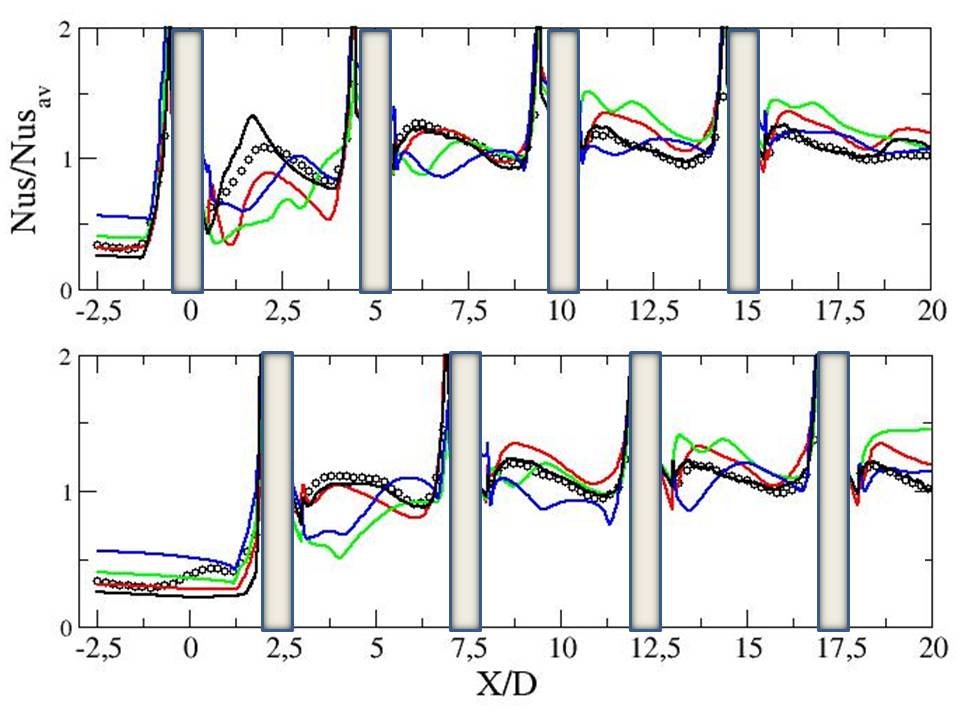
Figure ??: Local Nusselt number on the bottom wall - $Re_{D}=10000$ - top: Y=0, bottom: Y=1.25 - symb.: Exp. - black: LES - red: EBRSM - blue: Phi-model - green: kw-SST

Figure ??: Local Nusselt number on the bottom wall - $Re_{D}=30000$ - top: Y=0, bottom: Y=1.25 - symb.: Exp. - red: EBRSM - blue: Phi-model - green: kw-SST

---

Contributed by: Sofiane Benhamadouche — EDF

Front Page

Description

Test Case Studies

Evaluation

Best Practice Advice

References

© copyright ERCOFTAC 2024