UFR 4-18 Evaluation

Flow and heat transfer in a pin-fin array

Front Page

Description

Test Case Studies

Evaluation

Best Practice Advice

References

Evaluation

Comparison of CFD Calculations with Experiments

Discuss how well the CFD calculations of the assessment quantities compare with experiment and with one another. Present some key comparisons in the form of tables or graphical plots and, where possible, provide hyperlinks to the appropriate results database. Results with different turbulence models covering as wide a range as possible should be included in the discussion. However, if too many different calculation results are available (e.g. from workshops) do not present all the comparisons here. A selection should be made showing results only for the most typical and practically important models. Comprehensive comparisons can be made available via a link to the associated databases. Finally, draw conclusions on the ability of the models used to simulate the test case flow.

Global comparisons

Pressure loss coefficient

The following table gives the numerical values of the presure loss coefficient in Ames et al. experiment as well as those obtained in the main computations.

Figure ?? shows these values and compare them to existing correlations from the literature:

• Metzger et al. (1982) :

for $Re_{D}<10^{4}$, Failed to parse (syntax error): {\displaystyle f = 0.317 {Re_D}^{−0.132} } , for $Re_{D}>10^{4}$, Failed to parse (syntax error): {\displaystyle f = 1.76 {Re_D}^{−0.318}}

• Jacob (1938) :

$f=(0.25+0.1175/(P/D-1)^{1.08})Re^{-0.16}$

Note that the experimental results have an error of +/-2.5% at the higher Reynolds numbers.

Large Eddy Simulation shows a very good agreement with the correlations and Ames et al. experimental results. The relative error is equal to 1% end 3% for the two Reynolds numbers, respectively. for both computed Reynolds numbers. The EB-RSM shows a very satisfactory pressure loss coefficient at $Re_{D}=10000$ (1% error) but a worse pressure loss coefficient at $Re_{D}=30000$ (10% error). The kω-SST shows globally good results (7% and 6% errors) and the φ-model poorer results with an error of 17% and 12% for the two Reynolds numbers, respectively.

Wall resolved LES is then the best candidate to obtain almost perfect pressure loss coefficients in the present configuration. The EB-RSM five very good results at the lowest Reynolds number but a substantial error is observed at $Re_{D}=30000$. Although the kω-SST exhibits pretty good results, the physics of the present flow is not well captured and one can't rely on this model. The φ-model has to be avoided for the present configuration in order to compute the pressure loss coefficient.

Pressure loss coefficient values for the different computations

	Ames et al. $Re_{D}=3000$	LES3000	Ames et al. $Re_{D}=10000$	LES10000	EBRSM10000	PHI10000	kwSST10000	Ames et al. $Re_{D}=30000$	EBRSM30000	PHI30000	kwSST30000
Value	0.111	0.1076	0.095	0.0939	0.0963	0.0789	0.0883	0.07	0.0771	0.0615	0.0744
Error (%)	-	3	-	1	1	17	7	-	10	12	6

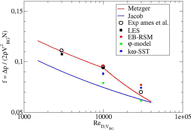
Figure ??: Pressure loss coefficient

Average Nusselt Number

The following table gives the numerical values of the average Nusselt numbers in Ames et al. experiment as well as those obtained in the main computations.

Figure ?? shows these values and compare them to existing correlations from the literature:

• Metzger et al. (1982) :

$Nus=0.079Re^{0.717}$

• Van Fossen (1982) :

$Nus=0.153*Re^{0.686}$

Note that the experimental results have an error of +/- 12%, +/-11.4%, and +/-10.5% for the 3 000, 10 000, and 30 000 Reynolds numbers, respectively, in the endwall regions adjacent to the pins and +/- 9% away from the pin.

Average Nusselt number on the bottom wall

	Ames et al. 3000	LES3000	Ames et al. 10000	LES10000	EBRSM10000	PHI10000	kwSST10000	Ames et al. 30000	EBRSM30000	PHI30000	kwSST30000
Value	22.1	21.6	54.1	48.6	48.1	37.6	33.1	111.5	114.8	93.3	72
Error (%)	-	2	-	10	11	30	39	-	3	16	35

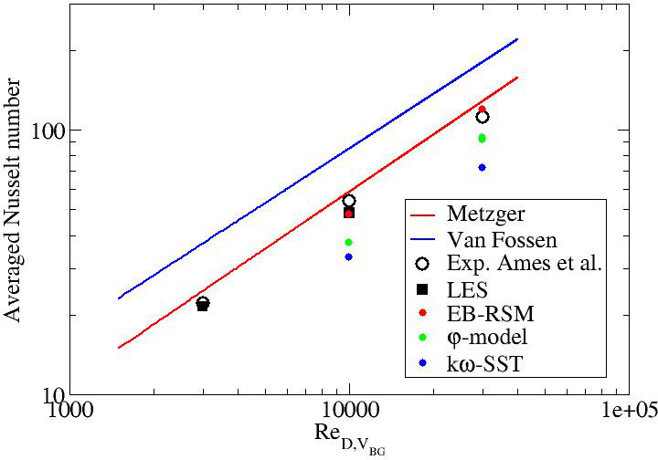
Figure ??: Averaged Nusselt number on the bottom wall

Local comparisons

Mean pressure coefficient

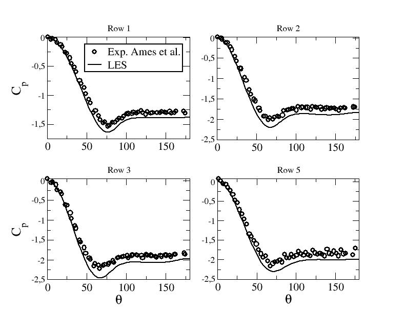
Figure ??: Pressure coefficient along the midline of the pins - LES at $Re_{D}=3000$

Figure ??: Pressure coefficient along the midline of the pins - LES and URANS computations at $Re_{D}=10000$

Figure ??: Pressure coefficient along the midline of the pins - URANS computations at $Re_{D}=30000$

Mean velocity profiles

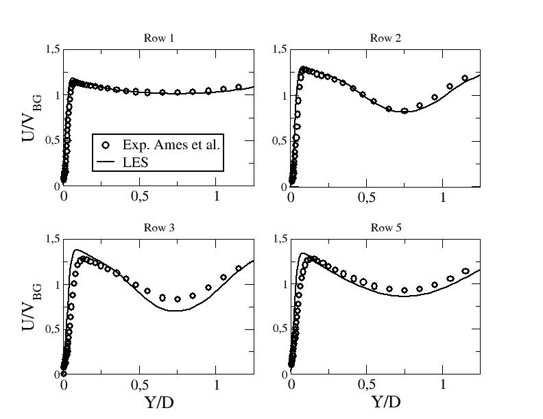
Figure ??: Mean stream-wse velocity component along line B - LES at $Re_{D}=3000$

Figure ??: Mean stream-wse velocity component along line B - LES and URANS computations at $Re_{D}=10000$

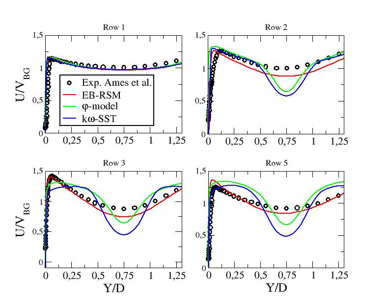
Figure ??: Mean stream-wse velocity component along line B - URANS computations at $Re_{D}=30000$

Figure ??: Mean stream-wse velocity component along line A1 - URANS computations at $Re_{D}=30000$

R.m.s. velocity profiles

Figure ??: R.m.s. of the stream-wise velocity component along line B - LES at $Re_{D}=3000$

Figure ??: R.m.s. of the stream-wise velocity component along line B - LES and URANS computations at $Re_{D}=10000$

Figure ??: Resolved and modelled contributions to the r.m.s. of the stream-wise velocity component along line B - URANS computations at $Re_{D}=10000$

Figure ??: R.m.s. of the stream-wise velocity component along line B - URANS computations at $Re_{D}=30000$

Figure ??: Resolved and modelled contributions to the r.m.s. of the stream-wise velocity component along line B - URANS computations at $Re_{D}=30000$

Figure ??: R.m.s. of the stream-wise velocity component along line A1 - URANS computations at $Re_{D}=30000$

Figure ??: Resolved and modelled contributions to the r.m.s. of the stream-wise velocity component along line A1 - URANS computations at $Re_{D}=30000$

Nusselt number on the bottom wall

Figure ??: Local Nusselt number on the bottom wall - LES computation at $Re_{D}=3000$ vs. experimental results from Ames et al.

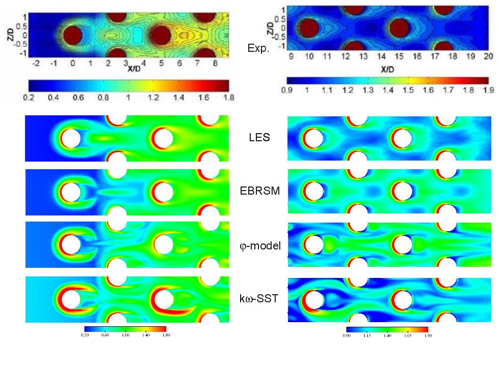
Figure ??: Local Nusselt number on the bottom wall - LES and URANS computations at $Re_{D}=10000$ vs. experimental results from Ames et al.

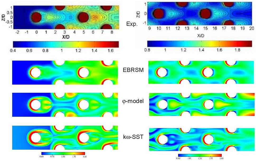
Figure ??: Local Nusselt number on the bottom wall - URANS computations at $Re_{D}=30000$ vs. experimental results from Ames et al.

Figure ??: Local Nusselt number on the bottom wall - $Re_{D}=3000$ - top: Y=0, bottom: Y=1.25 - symb.: Exp. - black: LES

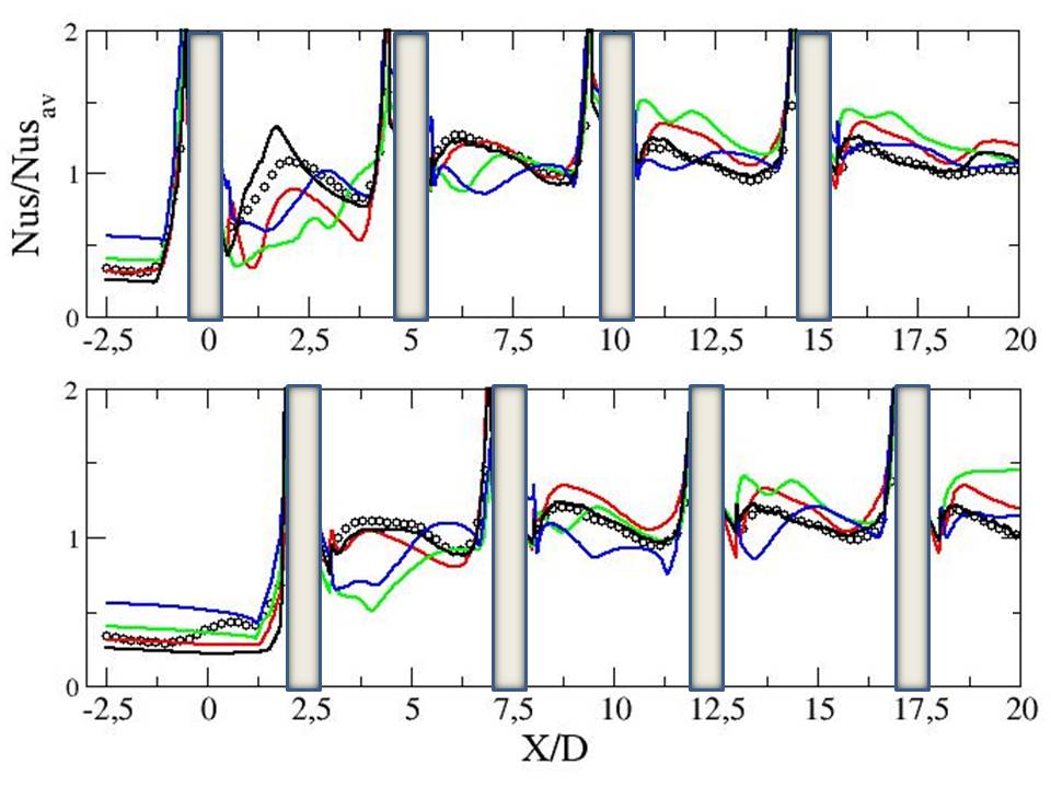
Figure ??: Local Nusselt number on the bottom wall - $Re_{D}=10000$ - top: Y=0, bottom: Y=1.25 - symb.: Exp. - black: LES - red: EBRSM - blue: Phi-model - green: kw-SST

Figure ??: Local Nusselt number on the bottom wall - $Re_{D}=30000$ - top: Y=0, bottom: Y=1.25 - symb.: Exp. - red: EBRSM - blue: Phi-model - green: kw-SST

---

Contributed by: Sofiane Benhamadouche — EDF

Front Page

Description

Test Case Studies

Evaluation

Best Practice Advice

References

© copyright ERCOFTAC 2024