Simple room flow

Underlying Flow Regime 4-11 © copyright ERCOFTAC 2004

Evaluation

Comparison of CFD calculations with Experiments

In comparing the CFD calculations with experiment, Run 03 is used as a 'base case' against which the effects of the various modelling refinements are judged:

mesh dependence

inlet flow rate (Reynolds number variation)

inlet representation (momentum model versus fixed velocity inlet)

turbulence and near-wall modelling methods (standard k-ε versus RNG, standard wall functions versus two-layer approach).

Flow Pattern, 3.0ach (Run 03)

For the 3.0 ach case, calculations were carried out using a mesh with 92,128 computational cells, as shown in fig2-02.gif. A region of embedded mesh refinement was used around the diffuser and outlet in an attempt to improve mesh resolution.

The simulated flow pattern within the domain for 3.0 ach is illustrated in fig2-02vect.jpg. This shows velocity vectors on the vertical symmetry plane and on a horizontal plane just below the ceiling. The ventilation air from the diffuser impinges at an angle on the ceiling of the test room. As the jet flows along the ceiling towards the far wall it spreads laterally, and when it impinges on the far wall it flows down the wall and along the floor, returning to the diffuser wall and flowing out through the outlet. This sets up a large recirculation vortex within the room, as shown by the velocity vectors on the symmetry plane.

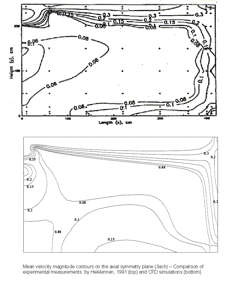
A comparison between the measured and computed velocity magnitude contours on the symmetry plane is given in fig2-03.jpg. The flow field is, on the whole, relatively well reproduced by the computations, with good qualitative predictions, and quantitative agreement to within a factor of around 2 in most of the domain. Close examination of these contour plots reveals the low flow velocities within the bulk of the room. This is a feature of most internal ventilation flows and is particularly relevant for the 1.5 and 3.0 ach experiments considered here.

Velocity Profiles, 3.0ach (Run 03)

Profiles of the mean velocity turbulence measured by Fontaine et al. (1991) in their model scale experiments are compared with the predicted profiles in fig2-05-ve.jpg (mean), fig2-05-te.jpg (turbulence), in the x, y and z directions at the centre of the room. Reasonably good agreement is demonstrated for the axial and vertical profiles, but less satisfactory results are achieved for the profile across the width of the room.

fig2-06.gif shows the velocity decay of the wall jet along the ceiling. The poor agreement is attributed to the coarseness of the mesh in the jet region and to the inadequacies of the diffuser model. However, it is evident that, despite this locally poor agreement, the flow field within the bulk of the domain is well reproduced by the computations.

Variation of inlet flow rate (1.5ach run)

In addition to the 3.0ach calculations, a computation was also carried out for the 1.5 ach case. In view of the lower flow rate, a coarser mesh was adopted for these calculations. The revised mesh used 67,488 computational cells. This mesh is similar in the interior of the domain to that used for the 3.0 ach case but is coarser near the walls. The reason for coarsening the mesh at the wall was to maintain an appropriate y+ value for the application of the wall function.

Unlike the 3.0ach case, where a large amount of data was available, only contours of the mean velocity magnitude on the symmetry plane are available for this case. fig2-07.jpg compares the calculated contours with the measurements of Lemaire (1992) The overall flow structure and the velocity levels within the room appear to be reasonably well reproduced.

Bulk Flow Parameters

Bulk flow parameters (as defined in the description of the study test case section) have been averaged over the occupied zone, and compared with the measured values in Table 2. The comfort of occupants within ventilated spaces is a function of both the mean velocity (U_m) and r.m.s turbulence (U_t) velocity components. Results can also be usefully presented in terms of U_mod, the r.m.s. of the total fluctuating velocity (where )

Table 2 Comparison of Measured and Computed Bulk Flow Parameters

It can be seen from this table that the mean velocities are slightly under-predicted and the turbulent velocity is over-predicted. This result is not surprising, in view of the fact that a high Reynolds number turbulence model has been used, when in fact the Reynolds number, based on individual inlet nozzle diameter and flow speed, is around 1600-3000. The alternative strategy would be to use a low Reynolds number turbulence model, but this would require a significantly refined mesh, with the associated overhead of very high computational costs.

Mesh Dependence

In addition to the computations described above for 3.0 ach, a series of calculations was also carried out on progressively finer meshes. In total, three different meshes were used:

(i) 15,120 cells (2l x 24 x 30);

(ii) 39,600 cells (33 x 30 x 40);

(iii) 92,128 cells (40 x 38 x 50), with embedded mesh refinement.

In principle, a mesh dependency study is a relatively simple experiment to conduct, given sufficient computing power. In practice, however, the mesh dependency study proved rather more difficult to conduct, primarily because of the difficulties experienced in controlling the near-wall cell distance and hence the y+ value (the calculations were conducted using the high Reynolds number k-ε turbulence model, and the no-slip wall conditions were imposed using a wall function).

With the low flow velocities in the test room, the friction velocity is low on test room walls and floor. Therefore, in order to satisfy the lower limit on y+, the mesh had to be relatively coarse. Typically, the first grid node was 0.126m distant from the floor.

To illustrate the effect of progressive mesh refinement on the solution, fig2-08.gif shows the variation of the axial velocity profile with the different meshes studied. It is clear that the solution is changing as the mesh resolution is improved, but the relative accuracy of each solution is difficult to determine from the plot presented. An objective measure of goodness of fit can be obtained, however, by calculating the Nomalised Mean Square Error (NMSE, Britter (1993)).

\displaystyle {NMSE={\frac {1}{N}}\sum {\frac {(X_{o}-X_{p})^{2}}{X_{o}X_{p}}}}

where N = no. of observations

X_o = observed values

X_p = predicted values

This statistic has been determined for the results shown in fig2-08.gif, using the 6 'interior' measurement points (i.e. ignoring the end points). The results are presented in Table 3, which demonstrates the superiority of the refined solution.

**Table 3 Goodness of fit for various mesh sizes**
Number of cells	15,120	39,600	92,128
NMSE	0.43	0.35	0.30

The effect of mesh resolution on the bulk properties has also been examined, and the results of this study are presented in Table 4. This shows that reasonable results may be obtained with a relatively coarse mesh, but that around 50,000-100,000 cells are required, in this case, before mesh dependence begins to diminish.

**Table 4 Effect of mesh resolution of the computed bulk flow parameters**
Average values [m/s]	Measured	Number of Computational Cells
Average values [m/s]	Measured	15,120	39,600	92,128
U_m	0.082-0.100	0.071	0.091	0.083
U_t	0.031-0.023	0.042	0.056	0.051
U_mod	0.089-0.103	0.082	0.107	0.097

The quantification of error can be undertaken systematically, as described by Roache (1994). Using results from a coarse and a fine solution mesh, he defines the Grid Convergence Index (GCI) as:

\displaystyle {GCI=3\vert \varepsilon \vert /(r^{N}-1)}

Where

\displaystyle {\varepsilon ={\frac {\phi _{c}-\phi _{f}}{\phi _{r}}}}

\displaystyle {r=(n_{f}/n_{c})\times 1/D}

and

D = dimensionality (= 3)

N = order of scheme (= 2 for SCFD)

n_i = number of grid cells

-c coarse grid

-f fine grid

&phi1;_i = predicted values of variable (coarse / fine)

φ_r = reference value of variable

The GCI is based upon a grid refinement error estimator derived from the theory of generalised Richardson Extrapolation and gives an estimate of the level of mesh dependence of a particular discretised solution. (It should be noted, however, that the predicted errors represent discretisation errors and not the overall solution accuracy). This analysis has been applied to grids used in Run 02 and Run 03, which have been compared respectively with Run 01 and Run 02. The discretisation error distribution is shown in fig2-09a.gif for Run02 and in fig2-09b.gif for Run 03. It is clear that the finer grid shows much smaller errors, in the region of 5% over most of the domain, whereas the coarser grid (Run 02) shows errors in excess of 10% over much of the domain.

Turbulence Models

In modelling room flows, the majority of CFD practitioners would adopt the standard k-ε turbulence model with wall functions, as presented above. In this study, two further simulations were carried out, one with the RNG extension of the k-ε model and one with the two-layer model. The RNG calculation was carried out using the same mesh as the standard k-ε model, but the two‑layer solution required a significantly finer mesh, as the momentum and turbulence equations are solved down to the wall, without the use of wall functions. As a consequence, there is a need to resolve the details of the boundary layer. The mesh used for this solution had 164,550 mesh cells with a minimum of 14 cells within the region 0<y+<150.

The RNG model had a minimal effect on the solution for this particular case. Its merits reportedly lie in its ability to improve solutions with strong flow re-circulation. Its inclusion requires minimal computational overhead and at worst it appears to have no effect on the solution whilst at its best could enhance a solution. In this case, although the flow is circulating within the room, the re-circulation is relatively weak, and its shape is well‑defined and constrained by the geometry. It is therefore hardly surprising that the RNG does not result in significant improvements in this case.

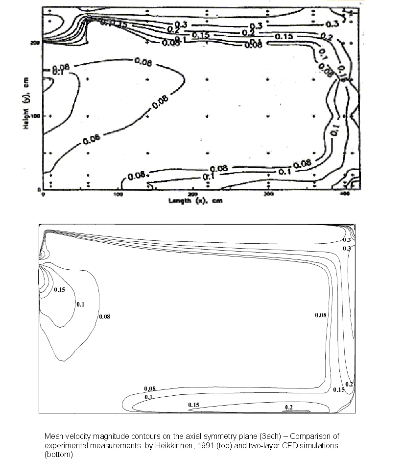
The use of the two-layer model did bring about a significant difference to the solution. This is illustrated in fig2-10.jpg, which again compares the computed and measured velocity contours on the symmetry plane. In particular, the velocity decay of the jet along the ceiling and floor and the thickness of the boundary layer on the far wall are predicted more accurately.

fig2-11.gif compares the computed and measured velocity profiles along the ceiling and shows the slightly increased accuracy in the ceiling jet. fig2-11.gif also compares the two‑layer solution with the previously presented profile for the k-ε solution. The error estimates, as discussed above, indicated that the maximum errors occurred in the diffuser inlet region. Thus, the improved solution may occur as a result of the increased mesh resolution within the jet rather than because of a better turbulence model.

Near the floor, the situation is quite different, since the flow velocities are very low in this region (approximately 0.1m/s) and the assumption of a high Reynolds number flow implicit in the use of the standard k-ε model and wall function approach is possibly invalid. The presence of low Reynolds number effects was noted by a number of the contributors to the IEA project. The two-layer model includes a near-wall modification which allows for low Reynolds number flow and it is therefore perhaps not surprising that the predictions improve with the use of this more appropriate turbulence model. This improvement was, however, achieved at a cost; the level of mesh resolution required is significantly greater than with the k-ε model and the convergence is therefore both more difficult to achieve and computationally more expensive.

Contributors: Steve Gilham; Athena Scaperdas - Atkins