UFR 3-35 Evaluation

Cylinder-wall junction flow

Front Page

Description

Test Case Studies

Evaluation

Best Practice Advice

References

Evaluation

For the evaluation of the numerical and experimental data sets in the symmetry plane upstream of a wall-mounted cylinder the following quantities are presented:

• the streamlines
• the location of the characteristic flow structures
• selected vertical and horizontal profiles of the mean velocity components $\langle u\rangle$ and $\langle w\rangle$ as well as the Reynolds stresses $\langle u'_{i}u'_{j}\rangle$ and the turbulent kinetic energy $\langle k\rangle$
• the contour plots of the turbulent kinetic energy and its buget terms such as production, diffusive transport, dissipation, and mean convection
• horizontal profiles of the pressure coefficient $c_{\mathrm {p} }(x)$, and the friction coefficient $c_{\mathrm {f} }(x)$

Streamlines

The streamlines of the PIV and the LES data agree well according to Fig. 6. The plots are superimposed by the normalized magnitude of the velocity field in the symmetry plane, thus $||{\vec {U}}||={\sqrt {\langle u^{2}\rangle +\langle w^{2}\rangle }}/u_{\mathrm {b} }$. The approaching turbulent boundary layer is redirected downwards at the flow facing edge of the cylinder caused by a vertical pressure gradient. This downflow reaches the bottom plate of the flume at the stagnation point S3. Here, it is redirected (i) in the out-of-plane direction bending around the cylinder; (ii) towards the cylinder rolling up and forming the corner vortex V3; and (iii) in the upstream direction accelerating and forming a wall-parallel jet. The jet accelerates and exerts a large wall-shear stress on the bottom plate (see Fig. cf). Parts of the downflow form the horseshoe vortex V1. Upstream of this vortex system, the approaching flow is blocked and causes a saddle point S1 with zero velocity magnitude.

Fig. 6 a) Streamlines of time-averaged flow field superimposed by the in-plane velocity magnitude $||{\vec {U}}_{\mathrm {PIV} }||={\sqrt {\langle u^{2}\rangle +\langle w^{2}\rangle }}/u_{\mathrm {b} }$

Fig. 6 b) Streamlines of time-averaged flow field superimposed by the in-plane velocity magnitude $||{\vec {U}}_{\mathrm {LES} }||={\sqrt {\langle u^{2}\rangle +\langle w^{2}\rangle }}/u_{\mathrm {b} }$

Location of the characteristic flow structures

The position of the characteristic flow structures highlighted in the streamline plots is listed in the following table

Tab. 3: Position of flow structures

	PIV		LES
	$x/D$	$z/D$	$x/D$	$z/D$
S1	$-0.788$	$0.03$	$-0.843$	$0.037$
S2	$-0.918$	$0$	$-1.1$	$0$
S3	$-0.533$	$0$	$-0.534$	$0$
S4	$-0.507$	$0.036$	$-0.50$	$0.04$
V1	$-0.697$	$0.051$	$-0.735$	$0.06$
V3	$-0.513$	$0.017$	$-0.513$	$0.02$

Horizontal and vertical profiles of the velocity components and Reynolds stresses

The vertical profiles are extracted at the following positions with respect to the time-averaged position of the horseshoe vortex (see Fig. 7).

Fig. 7: Position of vertical profiles in the flow

Since the flow structure of the LES and the PIV is slightly different, we use an adjusted $x-$coordinate, in order to compare the data at the same position in the flow. The coordinate is defined as follows (Schanderl 2018):

$x_{\mathrm {adj} }={\frac {x-x_{\mathrm {Cyl} }}{x_{\mathrm {Cyl} }-x_{\mathrm {V1} }}}$,

with $x_{\mathrm {Cyl} }=-0.5D$, such that $x_{\mathrm {adj} }=-1.0$ represents the time-averaged location of the horseshoe vortex centre $x_{\mathrm {V1} }$.

Fig. 8: Vertical profiles of the streamwise velocity component $\langle u(z)\rangle /u_{\mathrm {b} }$

The vertical velcoity profiles $u(z)$ are presented at the selected locations in Fig. 8. The wall-parallel jet starts to develop from S3 on and the flow accelerates. At $x_{\mathrm {adj} }=-0.25$, a near-wall velocity peak appears, which becomes more pronounced in the upstream direction (see $x_{\mathrm {adj} }=-0.5$). In this region, the wall-shear stress reaches on the one hand its maximum value and on the other hand reveals a plateau-like shape (this is shown and discussed later, see Fig. 22). This means that the largest values of the gradient ${\frac {\partial \langle u\rangle }{\partial z}}$ appear. Underneath the horseshoe vortex, the flow decelerates and the near-wall-peak of the velocity lifts from the bottom plate and becomes less distinct. Further upstream, the near-wall peak of the streamwise velocity disappears as the wall-parallel jet fades out. Due to the evaluation of the PIV images by an interrogation-window-based cross correlation, the strong gradient ${\frac {\partial \langle u\rangle }{\partial z}}$ at the wall cannot be fully resolved, and therefore, the near-wall peak of the streamwise velocity is damped in the experimental data.

Fig. 9: Vertical profiles of the Reynolds stresses $\langle u_{i}'u_{j}'(z)\rangle /u_{\mathrm {b} }^{2}$ and the turbulent kinetic energy $\langle k(z)\rangle =0.5(\langle u'^{2}\rangle +\langle w'^{2}\rangle )/u_{\mathrm {b} }^{2}$

The vertical profiles of the Reynolds stresses and the resulting turbulent kinetic energy comprising only streamwise and vertical fluctuating velocity components is presented in Fig. 9 at $x_{\mathrm {adj} }=-1.5$, $x_{\mathrm {adj} }=-1.0$, and $x_{\mathrm {adj} }=-0.5$. The accelerating jet is again indicated by a near wall peak of the $\langle u'u'\rangle$ stress, while the horseshoe vortex leaves its footprint in the stresses $\langle u'u'\rangle$ and $\langle w'w'\rangle$ as (local) peak at $z_{\mathrm {V1} }/D$. The shear stress distribution $\langle u'w'\rangle$ inside the wall-parallel jet is negative (in average) according to the average flow direction. The experimental and numerical data agree with each other both in amplitude as well as in shape. Again, the quality of the PIV data near the wall is undermined by the strong gradients being evaluated using interrogation windows.

Fig. 10: Horizontal profiles of the vertical velocity component $\langle w(x)\rangle /u_{\mathrm {b} }$ at the height $z_{\mathrm {V1} }/D$

Analysing the profile of the vertical velocity component $\langle w(x)\rangle$ along the $x-$axis at the height of the horseshoe vortex (see Fig. 10), reveals on the one hand the clockwise rotation of the vortex, and on the other hand two minima between the horseshoe vortex and the cylinder. At $x_{\mathrm {adj} }\approx -0.1$, the peak in the downwards directed flow stems from the downflow, while the second local minimum at approximately $x_{\mathrm {adj} }=-0.65$ represents the downwards rotation of the horseshoe vortex. Both data sets agree well in shape. However, the LES data indicate higher amplitudes in general, as the stagnation point at the cylinder front at which the approach flow is deflected and evolving the downflow, is located at the water level in the LES. Whereas it was shifted downwards in our experiment, due to the slat of acrylic glass at the water surface. This is, however, not an artefact as a bow wave (surface roller) would evolve in this area if this slat was not present according to e.g. Melville 2008. Therefore, the downwards deflected part of the flow is smaller in the experiment and therefore, the HV system becomes smaller, too.

Fig. 11: Horizontal profiles of the Reynolds stresses $\langle u_{i}'u_{j}'(x)\rangle /u_{\mathrm {b} }^{2}$ and the turbulent kinetic energy $\langle k(x)\rangle =0.5(\langle u'^{2}\rangle +\langle w'^{2}\rangle )/u_{\mathrm {b} }^{2}$ at the height $z_{\mathrm {V1} }/D$

The Reynolds stresses $\langle u_{i}'u_{j}'\rangle$ and the turbulent kinetic energy $\langle k\rangle$ are shown in Fig. 11 at the height of the horseshoe vortex and reveal similar distributions for the PIV and LES results. At the centre of the vortex, the normal stresses, and consequently the turbulent kinetic energy as well, reveal a peak, which wears off in the up- and downstream direction. In addition, the downflow close to the cylinder surface generates stresses as well. The shear stress plays a minor role in the region between the cylinder and the horseshoe vortex, while it becomes negative upstream of the horseshoe vortex indicating the interference of the approaching flow with the horseshoe vortex.

Distribution of turbulent kinetic energy and its budgets terms: production, diffusive transport, dissipation and convection

Turbulent kinetic energy

Fig. 12 a) Turbulent kinetic energy $\langle k_{\mathrm {PIV} }\rangle =0.5(\langle u'^{2}\rangle +\langle w'^{2}\rangle )/u_{\mathrm {b} }^{2}$

Fig. 12 b) Turbulent kinetic energy $\langle k_{\mathrm {LES} }\rangle =0.5(\langle u'^{2}\rangle +\langle w'^{2}\rangle )/u_{\mathrm {b} }^{2}$

The spatial distribution of the time-averaged in-plane turbulent kinetic energy $\langle k\rangle =0.5(\langle u'^{2}\rangle +\langle w'^{2}\rangle )/u_{\mathrm {b} }^{2}$ reveals on the one hand the well-known c-shaped structure (e.g. Paik 2007) with the largest amplitude at the centre of the horseshoe vortex stemming from vertical fluctuations induced by the horizontal oscillations of the horseshoe vortex. The lower branch of the c-shape contains mainly streamwise (horizontal) fluctuations linked to the dynamics of the wall-parallel jet. On the other hand, the experimental and numerical data sets show high similarity and agree well with each other, as the peak amplitude is approximately the same: $\langle k_{\mathrm {PIV} }\rangle =0.074u_{\mathrm {b} }^{2}$; $\langle k_{\mathrm {LES} }\rangle =0.079u_{\mathrm {b} }^{2}$. The black circle marks the centre of the horseshoe vortex.

The budget equation of the turbulent kinetic energy is the balancing sum of the production $P$, the diffusive transport term $\nabla T$, the dissipation $\epsilon$, and the mean convection $C$. In case of the LES data, these terms were calculated using the entire three dimensional velocity vector and the corresponding fluctuations. However, the influcence of the out-of-plane component Failed to parse (unknown function "\math"): {\displaystyle v <\math> is small due to symmetry (Schanderl et al. 2017). <math> 0 = P + \nabla T - \epsilon + C } ,

while $P=-\langle u_{i}'u_{j}'\rangle {\frac {\partial \langle u_{i}\rangle }{\partial x_{j}}}$,

$T=\underbrace {-{\frac {1}{2}}\langle u_{i}'u_{j}'u_{j}'\rangle } _{\text{turbulent fluctuations}}\underbrace {-{\frac {1}{\rho }}\langle u_{i}'p'\rangle } _{\text{pressure transport}}\underbrace {+2\nu \langle u_{j}'s_{ij}\rangle } _{\text{viscous diffusion}}$,

$\epsilon =2\nu \langle s_{ij}s_{ij}\rangle$, and $s_{ij}={\frac {1}{2}}\left({\frac {\partial u_{i}'}{\partial x_{j}}}+{\frac {\partial u_{j}'}{\partial x_{i}}}\right)$ as the fluctuating rate-of-strain tensor,

and $C=-{\frac {\partial k}{\partial t}}-\langle u_{i}\rangle {\frac {\partial k}{\partial x_{i}}}$.

The individual terms of the budget equation of the TKE are normalized by $D/u_{\mathrm {b} }^{3}$ and presented in the following part:

Production of turbulent kinetic energy

Fig. 13 a) Production of turbulent kinetic energy $P_{\mathrm {PIV} }=-\langle u_{i}'u_{j}'\rangle {\frac {\partial \langle u_{i}\rangle }{\partial x_{j}}}\cdot D/u_{\mathrm {b} }^{3}$

Fig. 13 b) Production of turbulent kinetic energy $P_{\mathrm {LES} }=-\langle u_{i}'u_{j}'\rangle {\frac {\partial \langle u_{i}\rangle }{\partial x_{j}}}\cdot D/u_{\mathrm {b} }^{3}$

Fig. 13 a) and b) show the TKE production using the PIV and LES results, respecively. The main region of positive production of turbulent kinetic energy can be found upstream of the centre of the hoseshoe vortex (black circle) and inside the wall-parallel jet. The amplitude of both data sets is about $0.3u_{\mathrm {b} }^{3}/D$ in the region of the horseshoe vortex, while the LES data resolve the TKE production in the jet in more detail than the PIV data. The amplitudes here are $P_{\mathrm {LES} }\approx 0.4u_{\mathrm {b} }^{3}/D$ and $P_{\mathrm {PIV} }\approx 0.2u_{\mathrm {b} }^{3}/D$. The oscillations of the horseshoe vortex are responsible for causing fluctuations, which in turn produce turbulent kinetic energy.

From the stagnation point S3 onwards in the upstream direction, the TKE production is negative, meaning that inside the accelerating jet TKE is transferred into mean kinetic energy. When the jet decelerates at about $x=-0.7D$, the jet becomes more unstable, fluctuations occur, and therefore, $P$ becomes positive.

Diffusive transport of turbulent kinetic energy

The diffusive transport of TKE is presented in Fig. 14 and can be split up into three individual terms: the transport due to turbulent fluctuations, due to pressure fluctuations, and due to viscous diffusion. Since the pressure in general is not contained in the PIV data, the velocity-pressure correlations, which are required to obtain the transport due to pressure, cannot be calculated, as well. Therefore, we present the three terms individually if available.

Fig. 14 a) Diffusive transport of turbulent kinetic energy due to turbulent fluctuations $\nabla T_{\mathrm {turb,PIV} }=-{\frac {1}{2}}{\frac {\partial \langle u_{i}'u_{j}'u_{j}'\rangle }{\partial x_{i}}}\cdot D/u_{\mathrm {b} }^{3}$

Fig. 14 b) Diffusive transport of turbulent kinetic energy due to turbulent fluctuations $\nabla T_{\mathrm {turb,LES} }=-{\frac {1}{2}}{\frac {\partial \langle u_{i}'u_{j}'u_{j}'\rangle }{\partial x_{i}}}\cdot D/u_{\mathrm {b} }^{3}$

The distribution of the turbulent transport shows a similar structure as the one of the production. In the region of large positive TKE production, we observe a large negative transport. In particular close to the wall at $x=-0.75D$, the large production of $0.4u_{\mathrm {b} }^{3}/D$ is nearly balanced by the turbulent transport $T_{\mathrm {turb,LES} }\approx 0.35u_{\mathrm {b} }^{3}/D$.

Positive transport indicates that TKE is transported towards these regions. They can be found above the centre of the horseshoe vortex. Accroding to Apsilidis et al. (2015), vertical eruptions from the wall occur here, which coincides with our observations.

Fig. 15 Diffusive transport of turbulent kinetic energy due to pressure fluctuations $\nabla T_{\mathrm {press,LES} }=-{\frac {1}{\rho }}{\frac {\partial \langle u_{i}'p'\rangle }{\partial x_{i}}}\cdot D/u_{\mathrm {b} }^{3}$

Fig. 16 Diffusive transport of turbulent kinetic energy due to viscous diffusion $\nabla T_{\mathrm {visc,LES} }=2\nu {\frac {\partial \langle u_{j}'s_{ij}\rangle }{\partial x_{i}}}\cdot D/u_{\mathrm {b} }^{3}$

The pressure fluctuations (Fig. 15) play an important role in the diffusive TKE-transport. In some regions, the transport terms $\nabla T_{\mathrm {turb} }$ and $\nabla T_{\mathrm {press} }$ cancel each other while the horseshoe vortex oscillates in the horizontal direction according to the alternation of the back-flow and zero-flow mode. While the horseshoe vortex moves towards the cylinder to a region with a downwards directed flow in average (Failed to parse (unknown function "\math"): {\displaystyle \langle w \rangle <0<\math>), the vortex core with an instantaneous zero <math> w-} velocity induces that the corresponding fluctuation $w'$ becomes positive. Therefore, the turbulent transport becomes negative in total, and the transport due to pressure fluctuations become positve as $p'<0$ in the vortex centre (low pressure), resulting in a mutual balance.

The transport of TKE due to viscous diffusion shows an increased negative transport only close to the wall (see (Fig. 16), which is intuitive as viscous effects increase towards the wall in turbulent flows. In the remaining part, however, the amplitude of $\nabla T_{\mathrm {visc} }$ is below $|0.05|u_{\mathrm {b} }^{3}/D$, and therefore, the contribution of this term to the TKE transport around the horseshoe vortex is of minor importance.

Dissipation of turbulent kinetic energy

The dissipation is the sink term in the budget of the TKE transport equation, as the TKE was produced and transported by $P$ and $\nabla T$, respectively, and is dissipated into heat by $\epsilon$. The dissipation is positive by definition, and therefore, it appears with a negive sign in the budget equation. In the LES data, the modelled dissipation due to subgird stresses is included and was quantified to be approximately one third of the total dissipation rate. Fig. 17 shows the dissipation rate calculated from PIV and LES data.

Fig. 17 a) Dissipation of turbulent kinetic energy $\epsilon _{\mathrm {PIV} }=2\nu \langle s_{ij}s_{ij}\rangle \cdot D/u_{\mathrm {b} }^{3}$

Fig. 17 b) Dissipation of turbulent kinetic energy $\epsilon _{\mathrm {LES} }=2\nu \langle s_{ij}s_{ij}\rangle \cdot D/u_{\mathrm {b} }^{3}$

The distribution of the dissipation shows a similar c-shaped structure as the TKE and the production term $P$ due to the horizontal oscillations of the vortex. Three regions with a high dissipation rate can be located: (i) around the centre of the horseshoe vortex; (ii) underneath the horseshoe vortex inside the wall-parallel jet; and (iii) at the corner vortex V3. The amplitude of the measured dissipation rate exceeds the one stemming from the LES data due to measurement noise undermining the quality of the instantaneous fluctuating velocity gradients. The spatial resolution of the PIV was anyway too coarse to estimate the dissipation correctly such that we did not apply any correction to the experimental data, and used the data as a qualitative comparison rather than a quantitative one. However, the dissipation rate and the production of the TKE do not cancel each other out as the maximum amplitude in the centre of the horseshoe vortex is $\epsilon _{\mathrm {LES} }=0.066u_{\mathrm {b} }^{3}/D$, which is approximately one third of the production here. Furthermore, the maximum value of the production is located upstream of the horseshoe vortex indicating the role of the transport of small-scale structures between the location of $P_{\mathrm {max} }$ towards $\epsilon _{\mathrm {max} }$.

Mean convection of turbulent kinetic energy

Since we analyse a steady state flow, the time derivative becomes irrelevant and the mean convection reduces to $C=-\langle u_{i}\rangle {\frac {\partial k}{\partial x_{i}}}$.

Mean convection of turbulent kinetic energy $C_{\mathrm {PIV} }=-\langle u_{i}\rangle {\frac {\partial k}{\partial x_{i}}}\cdot D/u_{\mathrm {b} }^{3}$

Mean convection of turbulent kinetic energy $C_{\mathrm {LES} }=-\langle u_{i}\rangle {\frac {\partial k}{\partial x_{i}}}\cdot D/u_{\mathrm {b} }^{3}$

The approaching flow separates from the bottom wall of the flume, and consequently, becomes unstable with increasing fluctuations. Therefore, the TKE increases along the streamline, which is indicated by the negative mean convection upstream of the horseshoe vortex. The same applies for the wall-parallel jet. After the deflection at S3, the jet accelerates, which decreases TKE in the first place. When the jet starts to decelerate ($x\approx -0.63D$) the flow becomes more unstable and the TKE increases. Underneath the horsehsoe vortex, $C$ changes sign again and the TKE decreases further upstream.

Budget of turbulent kinetic energy

Finally, the sum of the above mentioned terms is presented as the total budget of the TKE. Since the PIV data cannot provide information concerning the pressure, the corresponding residual will not cancel out.

Residual of turbulent kinetic energy budget $R_{\mathrm {PIV} }=P+\nabla T_{\mathrm {turb} }-\epsilon +C\cdot D/u_{\mathrm {b} }^{3}$

However, when analysing the distribution and amplitude of the residual of the TKE budget obtained from PIV, it appears that the structure is similar to the one of $-\nabla T_{\mathrm {press,LES} }$. Therefore, the missing piece in the experimental data of this flow configuration is the contribution of the pressure fluctuations to the transport mechanisms of the TKE (Jenssen 2019).

Residual of turbulent kinetic energy budget $R_{\mathrm {PIV} }=P+\nabla T-\epsilon +C\cdot D/u_{\mathrm {b} }^{3}$

The residual of the LES data is small in wide regions $<|0.01|u_{\mathrm {b} }^{3}/D$. In particular around the horseshoe vortex, the residual is close to zero. Alone, along the cylinder surface and the bottom wall the budget does not fully balance. On the one hand, we assign the large errors to the spatial resolution of the grid in the horizontal direction, which was obviously too coarse to fully resolve the developing boundary layer at the cylinder surface. On the other hand, the remaining error in the TKE budget can be associated to a lack of statistics, which mainly corrupt the quality of the term $T_{\mathrm {turb} }=-{\frac {1}{2}}\langle u_{i}'u_{j}'u_{j}'\rangle$, as the triple correlations of the velocity are highly sensitive to the number of samples.

Horizontal profiles of the pressure coefficient $c_{\mathrm {p} }(x)$, and of the friction coefficient $c_{\mathrm {f} }(x)$

The pressure coefficient $c_{\mathrm {p} }$ is computed as:

$c_{\mathrm {p} }={\frac {\langle p\rangle }{{\frac {\rho }{2}}u_{\mathrm {b} }^{2}}}$,

while the friction coefficient $c_{\mathrm {f} }$ is determined as:

$c_{\mathrm {f} }={\frac {\langle \tau _{\mathrm {w} }\rangle }{{\frac {\rho }{2}}u_{\mathrm {b} }^{2}}}$.

The following plots were taken from the LES data only since the pressure is not contained in the PIV data and the spatial resolution in the experiment appeared to be too coarse to calculate the wall-shear stress, thus the friction coefficient, correctly. The first data point in the experimental data could be obtained at $z_{1}\approx 0.0036D\approx 10\mathrm {px}$. In the LES, the first grid point was at $z_{1}\approx 0.0005D$, which is about a factor of 7 finer than the experimental results.

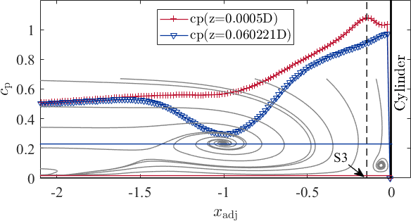
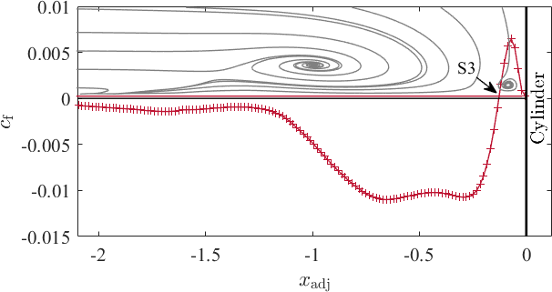
A streamline plot in light grey is given for the sake of better orientation in a qualitative sense showing the positions in the $z-$direction at which the profiles were extracted. The red symbols refer to the profiles near the wall indicated by the red solid line, whereas the blue symbols and the blue solid line refer to the profile at the height of the horseshoe vortex.

• 

  Pressure coefficient $c_{\mathrm {p} }$
• 

  Friction coefficient $c_{\mathrm {f} }$

According to the horizontal profile at the height of the first grid point, the pressure coefficient reaches a maximum due to the downflow impinging at the bottom of the flume at the stagnation point S3. The downflow is deflected in all directions forming an accelerating wall-parallel jet especially in the uptream direction. The acceleration is indicated by the decrease of the pressure coefficient. At $x_{\mathrm {adj} }=-1.0$, underneath the horseshoe vortex, the pressure coefficient shows a kink and decreases less significant than before.

Following the downflow in the vertical direction towards the bottom plate of the flume, the pressure increases with decreasing distance to the bottom. The pressure coefficient $c_{\mathrm {p} }$ increases likewise. Therefore, near the cylinder surface, the pressure coefficient shows a high amplitude at the height of the horseshoe vortex. Along a horizontal axis at $z_{\mathrm {V1} }=0.06D$, $c_{\mathrm {p} }$ decreases reaching its minimum value of about $0.3$ coinciding with the centre of the horseshoe vortex. Upstream of the horseshoe vortex, the horizontal profiles of the pressure coefficient coincide with each other irrespectively of the wall distance.

The accelerating wall-parallel jet is also perceptible in the distribution of the friction ceofficient $c_{\mathrm {f} }$, which was extracted at the first grid point. From the stagnation point S3 on, with zero wall-shear stress, the friction coefficient reveals a sharp peak underneath the foot vortex V3. In the upstream direction, the wall-shear stress increases due to the accelerating jet until a plateau is reached. Here, the friction coefficient is almost constant at $|c_{\mathrm {f} }|=0.01$, which represents the maximum absolute value. It should be noted that the maximum is not located underneahth the horseshoe vortex. The distribution of $c_{\mathrm {f} }$ is dominated by the wall-parallel jet rather than by the horseshoe vortex. Further upstream, the value of $c_{\mathrm {f} }$ is small but negative, indicating the fading near-wall jet pointing still in the upstream direction. Unlike Apsilidis et al. (2015), we could not observe a second vortex here.

Data sets for download

• PIV data: Media:UFR3-35_X_data.txt
• LES data: Media:UFR3-35_C_data.zip
• LES: friction coefficient $c_{\mathrm {f} }$ Media:UFR3-35_C_cf.txt
• How to read in the data as an example (MATLAB): Media:UFR3_35_read_data.m

The data are structured as follows:

• 2D plots of the PIV have $50\times 171(n\times m)$ data points
• 2D plots of the LES have $143\times 131(n\times m)$ data points
• The .txt files are reshaped such as each column has $n\cdot m$ entries
• The first 11 lines of the .txt files belong to the header, which are indicated by the #-symbol
• Each column corresponds to the following data and is comma separated

Tab. 4: Structure of data sets

Column number	1	2	3	4	5	6	7	8	9	10	11	12	13	14	15	16	17	18	19
PIV	$x_{\mathrm {adj} }$	${\frac {x}{D}}$	${\frac {z}{D}}$	${\frac {\langle u\rangle }{u_{\mathrm {b} }}}$	$-$	${\frac {\langle w\rangle }{u_{\mathrm {b} }}}$	${\frac {\langle u'u'\rangle }{u_{\mathrm {b} }^{2}}}$	$-$	${\frac {\langle w'w'\rangle }{u_{\mathrm {b} }^{2}}}$	$-$	${\frac {\langle u'w'\rangle }{u_{\mathrm {b} }^{2}}}$	$-$	$P{\frac {D}{u_{\mathrm {b} }^{3}}}$	$C{\frac {D}{u_{\mathrm {b} }^{3}}}$	$\nabla T_{\mathrm {turb} }{\frac {D}{u_{\mathrm {b} }^{3}}}$	$-$	$-$	$\epsilon {\frac {D}{u_{\mathrm {b} }^{3}}}$	$-$
LES	$x_{\mathrm {adj} }$	${\frac {x}{D}}$	${\frac {z}{D}}$	${\frac {\langle u\rangle }{u_{\mathrm {b} }}}$	${\frac {\langle v\rangle }{u_{\mathrm {b} }}}$	${\frac {\langle w\rangle }{u_{\mathrm {b} }}}$	${\frac {\langle u'u'\rangle }{u_{\mathrm {b} }^{2}}}$	${\frac {\langle v'v'\rangle }{u_{\mathrm {b} }^{2}}}$	${\frac {\langle w'w'\rangle }{u_{\mathrm {b} }^{2}}}$	${\frac {\langle u'v'\rangle }{u_{\mathrm {b} }^{2}}}$	${\frac {\langle u'w'\rangle }{u_{\mathrm {b} }^{2}}}$	${\frac {\langle v'w'\rangle }{u_{\mathrm {b} }^{2}}}$	$P{\frac {D}{u_{\mathrm {b} }^{3}}}$	$C{\frac {D}{u_{\mathrm {b} }^{3}}}$	$\nabla T_{\mathrm {turb} }{\frac {D}{u_{\mathrm {b} }^{3}}}$	$\nabla T_{\mathrm {press} }{\frac {D}{u_{\mathrm {b} }^{3}}}$	$\nabla T_{\mathrm {visc} }{\frac {D}{u_{\mathrm {b} }^{3}}}$	$\epsilon {\frac {D}{u_{\mathrm {b} }^{3}}}$	$c_{\mathrm {p} }$

---

Contributed by: Ulrich Jenssen, Wolfgang Schanderl, Michael Manhart — Technical University Munich

Front Page

Description

Test Case Studies

Evaluation

Best Practice Advice

References

© copyright ERCOFTAC 2019