Evaluation AC2-08: Difference between revisions
| Line 23: | Line 23: | ||
Comparing the efficiency functions (which is the main model parameter) the differences (marked with arrows in Fig.5.1 and 5.2) between the two formulations are small and hence the model uncertainty will not influence the results crucially. | Comparing the efficiency functions (which is the main model parameter) the differences (marked with arrows in Fig.5.1 and 5.2) between the two formulations are small and hence the model uncertainty will not influence the results crucially. | ||
====<span class="titlemark"> References==== | |||
<references/> | |||
<br> | <br> | ||
Revision as of 14:40, 11 January 2011
Premixed Methane-Air Swirl Burner (TECFLAM)
Application Challenge 2-08 © copyright ERCOFTAC 2011
In order to assess the simulation a comparison of the time averaged velocity, temperature and species distribution with experimental data is presented in this section. A more extensive evaluation can be found in Kuenne et al.[1] .
Comparison of CFD Results with Experimental Data
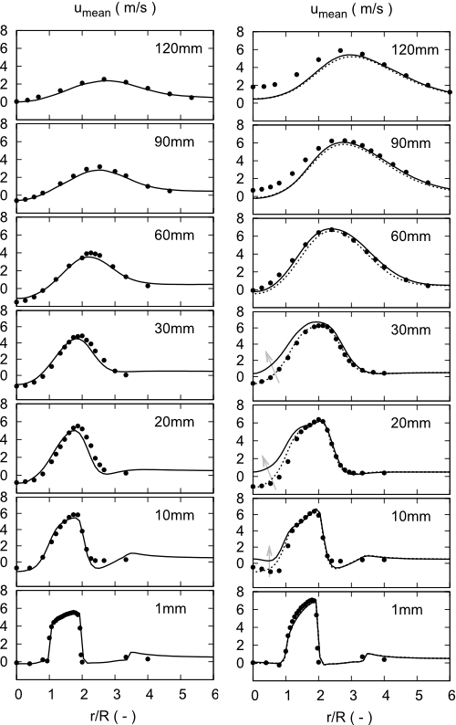
In Fig. 5.1 the simulation results of the axial velocity for the isothermal and reacting case are compared with experimental data. As is typical for this type of swirl flow, the velocity field starts to expand right after the nozzle exit, which produces a positive pressure gradient in the axial and radial direction, high enough to form a central recirculation zone as intended for flame stabilization. Overall the spreading of the turbulent swirling flow and the size and intensity of the recirculation zone are well predicted and an excellent agreement with the measurements can be observed in all axial planes for both cases. Comparing the isothermal and reacting case a strong acceleration of the velocity caused by the thermal expansion through the flame front can be observed which is accurately reproduced by the simulation.
In Fig. 5.2 the temperature and methane mass fraction are compared with experimental data. Since the flame is very sharp the distribution is almost completely caused by the flame-turbulence interaction resulting in a wide turbulent flame brush. Except that a small radial offset exists and the gradient at higher axial positions is slightly over predicted the temperature is well predicted by the simulation. The mean profile of the methane mass fraction reflects its consumption by the chemical reaction on the left and the mixing with the coflowing air on the right. At the higher axial positions the methane mass fraction exceeds the measurement indicating insufficient fuel consumption in the simulation.
Comparing the efficiency functions (which is the main model parameter) the differences (marked with arrows in Fig.5.1 and 5.2) between the two formulations are small and hence the model uncertainty will not influence the results crucially.
References
Contributors: Johannes Janicka (EKT), Guido Kuenne (EKT), Andreas Dreizler (RSM)

