AC 6-12 CFD Simulations
Steam turbine rotor cascade
Application Challenge 6-12 © copyright ERCOFTAC 2004
CFD Simulations
Overview of CFD Simulations
CFD simulations were carried out for inviscid flows using finite volume methods and grids of quadrilaterall cells (H type) or triangular cells by explicit modern (TVD central and upwind, ENO high order) methods or classical (Ron-Ho-Ni cell-vertex) methods and by implicit methods (TVD-Osher preconditioning and ENO second order implicit). The adaptivity of grids was used in explicit and implicit methods using triangular cells.
Numerical results are good in the vicinity of sonic line and in the downstream part considering shock waves, reflected shock waves, wakes (compared to experimental data using pressure distribution or field of Mach number isolines). Behind of the leading edge of the upper side of the profile, results achieved by triangular grid are better for any type of used method. Relatively good results were obtained for laminar viscous flow computed by the combination of finite volume (inviscid part) and finite element (viscous part) methods.
Convergence to the steady state was examined by log L2 − residual. Numerical and experimental results are compared using pressure and Mach number distribution along the profile surface with a very good agreement.
The Reynolds-Averaged Navier-Stokes (RANS) equations were solved by FLUENT 5 code using the RNG k-eps turbulence model for the Reynolds number Re = 1.5 x 10⁶. The obtained pressure distribution on the profile shows a very good agreement with experiment. The comparison of measured and computed energy losses was made as well.
Some disadvantage of the FLUENT code is that the used numerical procedure has not implemented downstream non-reflection boundary conditions.
Simulation Cases CFD1 and CFD2
Solution strategy
Case CFD1 is turbulent computation, case CFD2 is inviscid computation. Basic equations used in CFD1 and CFD2 computations are considered in conservative form (RANS and Euler equations respectively). For RANS computations we used additionally one- or two-equation models needed to compute turbulent viscosity. Finite volume methods were considered in both cases. For inviscid problem we used only our own software. For viscous computation FLUENT 5 was used.
The fluid flow in the cascade was solved as adiabatic compressible air flow using the commercial code FLUENT 5. Two turbulence models were used: RNG k-eps model and Spalart-Allmaras model. The RNG k-eps model was chosen for the application challenge. Wall functions were used as wall boundary conditions.
Computational Domain
We used as a computational domain one period or two periods:
a) with profile located inside of the domain and upper-lower boundary of the domain are lines where periodicity conditions are fulfilled.
b) with periodical boundaries and part of the boundary is also lower-upper part of a profile (profile is not located inside of the domain when one period is considered).
Boundary Conditions
Numerical simulations were made for the cascade section one and/or two blade passages. The upstream boundary was approximately one chord before the inlet plane of the cascade. The downstream boundary was situated in the distance 1.5 – 2 chords behind the outlet plane. At the inlet boundary, three quantities were given and one was extrapolated. The pressure was given at the outlet boundary. Periodical boundaries were used along the cascade passage. Wall functions were used as wall conditions in calculations made using the FLUENT code and the reflection principle was used in home-made software.
Application of Physical Models
Two physical models are used:
a) CFD1 – RANS with RNG k-ε turbulence model or one-equation Spalart-Allmaras model
b) CFD2 – Euler equations
In part a) all needed is given by code FLUENT 5, in part b) used boundary conditions are described above.
Numerical Accuracy
We compared several results for inviscid flows using high resolution different schemes (TVD, ENO,…) on different grids. We also have comparison of numerical and experimental results. The similar way was used for turbulent RANS computations.
CFD Results
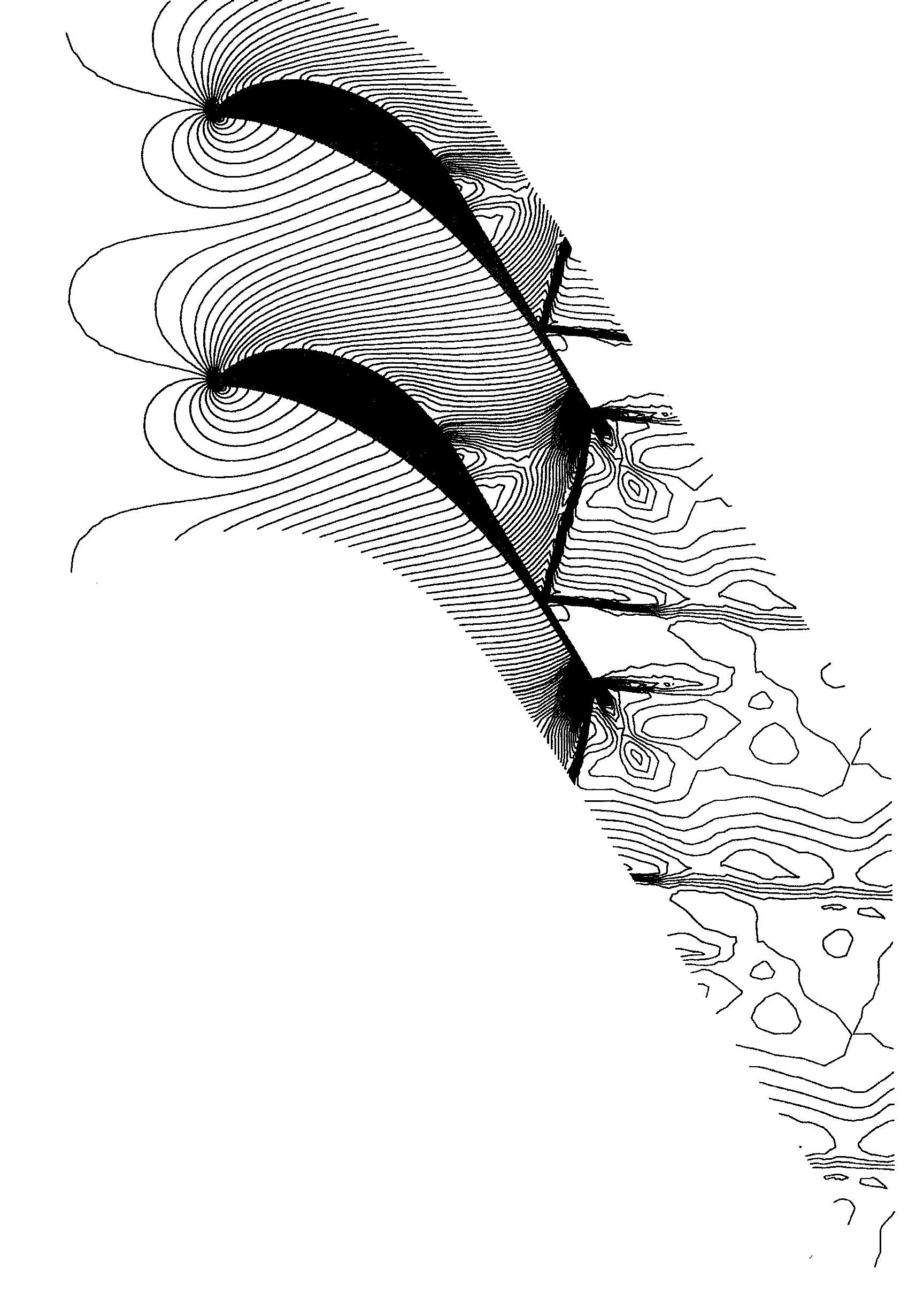
CFD1 Numerical simulation of the viscous flow the steam turbine rotor cascade: isolines of density ρ=f(x,y), pressure distribution on the blade, survey of relevant parameters
The files containing results with measured and evaluated parameters are given in Table EXP-B:
cfd11.jpg (flow field description by density isolines for M2is = 1.198)
cfd12.dat (survey of relevant data β1, i, M1, M2is, Re2is, M2, ζ, β2 and pressure distribution on the suction and pressure sides p/p0 vers. x/b)
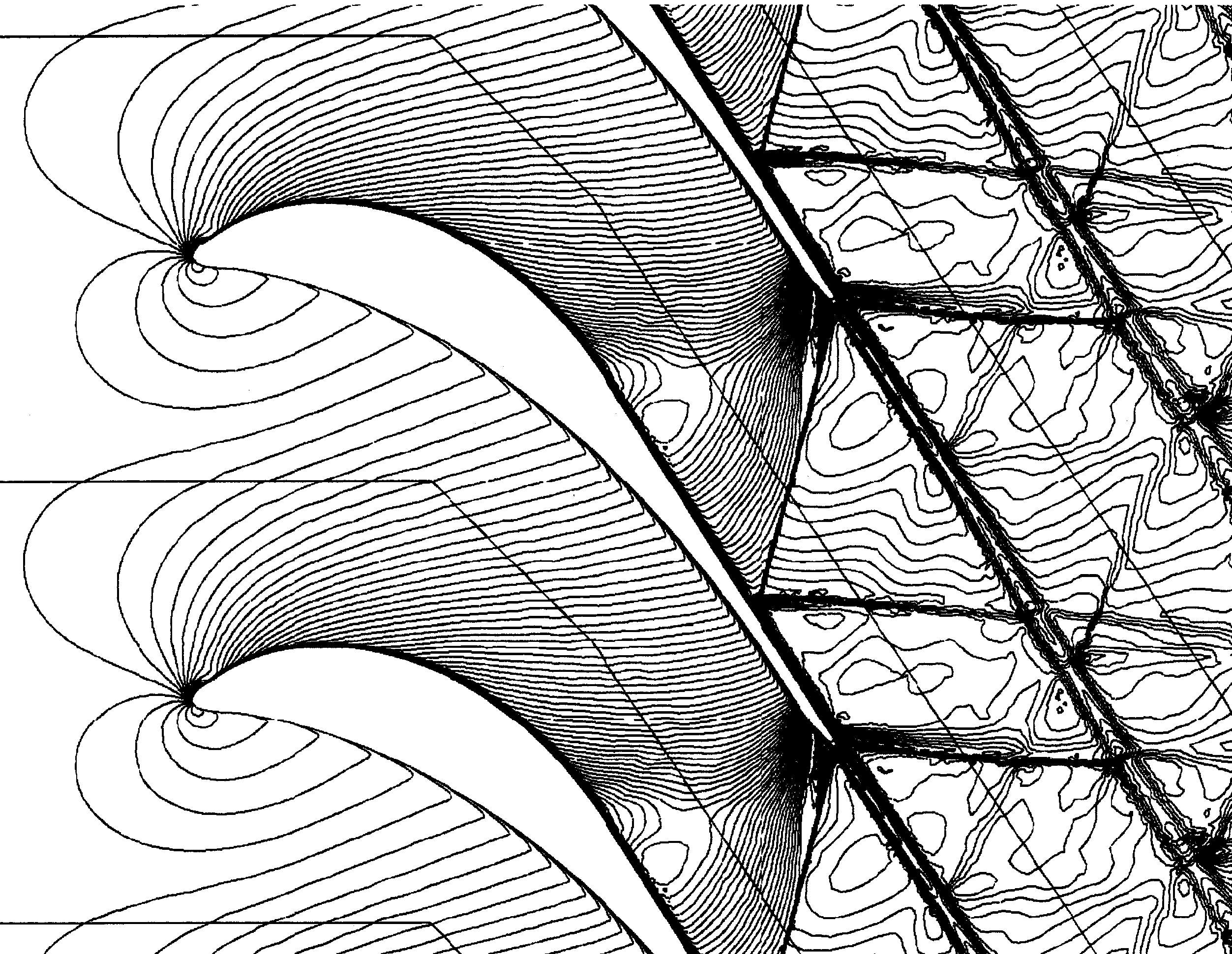
CFD2 Numerical simulation of the inviscid flow the steam turbine rotor cascade: isolines of Mach number M=f(x,y), pressure distribution on the blade, survey of relevant parameters
The files containing results with measured and evaluated parameters are given in Table EXP-B:
cfd21.jpg (flow field description by Mach number isolines for M2is = 1.198)
cfd22.dat (survey of relevant data β1, i, M1, M2is, β2 and pressure distribution on the suction and pressure sides p/p0 vers. x/b)
|
Name |
|
|
| ||||
|
|
|
|
|
|
|
|
|
|
CFD 1 |
|
|
|
|
|
|
|
|
CFD 2 |
|
|
|
|
|
|
|
|
|
|
survey of relevant parameters pressure distribution p/po=f(x/b) |
|
|
|
|
|
|
|
|
References
[1] Feistauer M., Felcman J. Theory and applications of numerical schemes for nonlinear convection-diffusion problems and compressible Navier-Stokes equations, Mathematics of Finite Elements and Applications, 175-194, Wiley, Chichester, 1997
[2] Fialová M., Hyhlík T., Kozel K., Šafařík P. Numerical analysis data on the transonic flow past the profile cascade SE 1050, Proc. of the Seminar “Topical Problems of Fluid Mechanics”, Institute of Thermomechanics, Prague, 45-48, 2001
[3] Fořt J., Fürst J., Halama J., Kozel K.: Numerical Solution of 2D and 3D Transonic Flows through a Cascade, Proc. of 4th International Symposium on Experimental and Computational Aerothermodynamics of Internal Flows (ed. R. Grundmann), Dresden, Vol.1., 231-240, 1999
[4] Fořt J., Huněk M., Kozel K., Lain J., Šejna M., Vavřincová M. Numerical simulation of steady and unsteady flow through plane cascades, Lecture Notes on Physics (eds. S.M. Desphande, S.S. Desai, R. Narasimha), Vol.453, 461-465, Springer, Berlin, 1995
[5] Matas R., Jůza Z., Riffault T. Some experiences with 2D numerical modelling of transonic profile cascade SE 1050, Proc. of the Colloquium “Fluid Dynamics”, Institute of Thermomechanics, Prague, 85-88, 2000
© copyright ERCOFTAC 2004
Contributors: Jaromir Prihoda; Karel Kozel - Czech Academy of Sciences