AC 6-08 CFD Simulations: Difference between revisions
David.Fowler (talk | contribs) |
m (Dave.Ellacott moved page Gold:AC 6-08 CFD Simulations to AC 6-08 CFD Simulations over redirect) |
||
| (15 intermediate revisions by 4 users not shown) | |||
| Line 1: | Line 1: | ||
{{AC|front=AC 6-08|description=AC 6-08 Description|testdata=AC 6-08 Test Data|cfdsimulations=AC 6-08 CFD Simulations|evaluation=AC 6-08 Evaluation|qualityreview=AC 6-08 Quality Review|bestpractice=AC 6-08 Best Practice Advice|relatedUFRs=AC 6-08 Related ACs}} | |||
{{AC|front=AC 6-08|description=AC 6-08 Description|testdata=AC 6-08 Test Data|cfdsimulations=AC 6-08 CFD Simulations|evaluation=AC 6-08 Evaluation|qualityreview=AC 6-08 Quality Review|bestpractice=AC 6-08 Best Practice Advice| | |||
| Line 19: | Line 18: | ||
Over the last years, calculations for the design speed were carried out with five different viscous 3D-solvers. These codes were: | Over the last years, calculations for the design speed were carried out with five different viscous 3D-solvers. These codes were: | ||
* VISIUN (commercial code developed at NREC) | |||
* STAGE3D (developed from Dawes’ structured 3D multiple-blade row NS solver). | |||
* CFX-TASCflow (commercial code supplied by AEA Technology, UK) | |||
* FLOWSIM (development of DLR from code NEWT) | |||
* FineTurbo (commercial code supplied by NUMECA International, Belgium) | |||
The main intention of performing CFD calculations was to find the global flow field structures and indications for necessary blade design changes that could lead to a further improvement of impeller efficiency. All codes used were capable of giving this information, but the simulations on different grids were unable to identify best practice guidelines for this case. The results presented here are new simulations carried out with CFX-TASCflow. | The main intention of performing CFD calculations was to find the global flow field structures and indications for necessary blade design changes that could lead to a further improvement of impeller efficiency. All codes used were capable of giving this information, but the simulations on different grids were unable to identify best practice guidelines for this case. The results presented here are new simulations carried out with CFX-TASCflow. | ||
Table 3-I, partially taken from Eisenlohr et al. [2], summarizes the main features of each code. | Table 3-I, partially taken from Eisenlohr et al. [2], summarizes the main features of each code. | ||
{| style="border-collapse: collapse" | {| style="border-collapse: collapse" | ||
| Line 112: | Line 113: | ||
Combination of multigrid and implicit residual averaging | Combination of multigrid and implicit residual averaging | ||
|} | |} | ||
Table CFD-A Overview of CFD simulations | Table CFD-A Overview of CFD simulations | ||
| Line 127: | Line 129: | ||
The geometry for the computational domain includes: | The geometry for the computational domain includes: | ||
<span lang="EN-US"><font face="Wingdings">§<span style="font: 7.0pt "Times New Roman""> | <span lang="EN-US"><font face="Wingdings">§<span style="font: 7.0pt "Times New Roman""> </span></font></span>the channel with one main and one splitter blade excluding the blade fillet radii at the hub, | ||
<span lang="EN-US"><font face="Wingdings">§<span style="font: 7.0pt "Times New Roman""> | <span lang="EN-US"><font face="Wingdings">§<span style="font: 7.0pt "Times New Roman""> </span></font></span>the casing and hub contour, including the spinner geometry and vaneless diffuser, and | ||
<span lang="EN-US"><font face="Wingdings">§<span style="font: 7.0pt "Times New Roman""> | <span lang="EN-US"><font face="Wingdings">§<span style="font: 7.0pt "Times New Roman""> </span></font></span>the blade tip clearance. | ||
The geometry of the main blade and the splitter blade are given in cartesian (and polar) coordinates. Note that the splitter blade is not yet rotated by half a pitch (i.e. 360°/(13+13) ). | The geometry of the main blade and the splitter blade are given in cartesian (and polar) coordinates. Note that the splitter blade is not yet rotated by half a pitch (i.e. 360°/(13+13) ). | ||
| Line 137: | Line 139: | ||
The blade tip clearance was assumed to be 0.5mm at the leading edge and 0.6mm at the trailing edge. As the exact value of the tip clearance is not known for sure, see discussion under section additional simulations have been carried out with an increased width to get an idea of the influence: | The blade tip clearance was assumed to be 0.5mm at the leading edge and 0.6mm at the trailing edge. As the exact value of the tip clearance is not known for sure, see discussion under section additional simulations have been carried out with an increased width to get an idea of the influence: | ||
• CFD1 original width (i.e. 0.5mm at LE; 0.6mm at TE) | |||
• CFD2 50% increase (i.e. 0.75mm at LE; 0.9mm at TE) | |||
• CFD3 100% increase (i.e. 1.0mm at LE; 1.2mm at TE) | |||
Available geometry files: | Available geometry files: | ||
• [[media:AC6-08_geo1.dat|geo1.dat]] coordinates (x,y,z and r,phi) of main blade | |||
• [[media:AC6-08_geo2.dat|geo2.dat]] coordinates (x,y,z and r,phi) of splitter blade (not yet rotated) | |||
• [[media:AC6-08_geo3.dat|geo3.dat]] coordinates (z,r) of hub | |||
• [[media:AC6-08_geo4.dat|geo4.dat]] coordinates (z,r) of shroud | |||
• [[media:AC6-08_geo5.dat|geo5.dat]] coordinates (z,r) of tip gap (CFD1) | |||
• [[media:AC6-08_geo6.dat|geo6.dat]] coordinates (z,r) of tip gap (CFD2) | |||
• [[media:AC6-08_geo7.dat|geo7.dat]] coordinates (z,r) of tip gap (CFD3) | |||
The computational domain has been modeled by | The computational domain has been modeled by | ||
• 160 nodes in the stream-wise direction<br /> (49 nodes for the inlet region; 70 nodes along main blade; 39 nodes along splitter blade; 43 nodes for the diffuser) | |||
• 66 nodes in the circumferential direction | |||
• 31 nodes from hub to tip, and | |||
• 6 nodes from tip to casing | |||
giving a total number of | giving a total number of 350,000 active nodes. | ||
=== Boundary Conditions === | === Boundary Conditions === | ||
Total-Pressure and Total-Temperature have been used as the inlet condition with the flow direction purely axial in the absolute frame of reference. For the k-ε turbulence model the turbulence level has been set to 5% and the viscosity ratio | Total-Pressure and Total-Temperature have been used as the inlet condition with the flow direction purely axial in the absolute frame of reference. For the k-ε turbulence model the turbulence level has been set to 5% and the viscosity ratio ν<sub>t</sub>/ν to 10. | ||
At the outlet either the average static pressure or the mass flow has been specified, depending on the position on the characteristic. Starting with a sufficiently small value (1.5E5Pa | At the outlet either the average static pressure or the mass flow has been specified, depending on the position on the characteristic. Starting with a sufficiently small value (1.5E5Pa – 2.2E5Pa) the outlet pressure has been increased. When the gradient dP/d[[Image:A6-08d30_files_image013.gif]] becomes too small, the outlet condition has been changed to a mass flow outlet condition and the mass flow stepwise decreased. As can be seen in Fig 3.1 the characteristic shows a smooth transition from the “pressure driven” to the “mass flow driven” leg of the characteristic. | ||
[[Image:A6-08d30_files_image015.gif]] | [[Image:A6-08d30_files_image015.gif]] | ||
| Line 231: | Line 233: | ||
<center>x</center> | <center>x</center> | ||
| style="width: 26.55pt; border-top: none; border-left: none; border-bottom: solid windowtext 1.0pt; border-right: solid windowtext 1.0pt; padding: 0cm 5.4pt 0cm 5.4pt" width="35" valign="top" | | | style="width: 26.55pt; border-top: none; border-left: none; border-bottom: solid windowtext 1.0pt; border-right: solid windowtext 1.0pt; padding: 0cm 5.4pt 0cm 5.4pt" width="35" valign="top" | | ||
<center> | <center> </center> | ||
| style="width: 26.6pt; border-top: none; border-left: none; border-bottom: solid windowtext 1.0pt; border-right: solid windowtext 1.0pt; padding: 0cm 5.4pt 0cm 5.4pt" width="35" valign="top" | | | style="width: 26.6pt; border-top: none; border-left: none; border-bottom: solid windowtext 1.0pt; border-right: solid windowtext 1.0pt; padding: 0cm 5.4pt 0cm 5.4pt" width="35" valign="top" | | ||
<center>x</center> | <center>x</center> | ||
| Line 264: | Line 266: | ||
CFD2 | CFD2 | ||
| style="width: 23.95pt; border-top: none; border-left: none; border-bottom: solid windowtext 1.0pt; border-right: solid windowtext 1.0pt; padding: 0cm 5.4pt 0cm 5.4pt" width="32" valign="top" | | | style="width: 23.95pt; border-top: none; border-left: none; border-bottom: solid windowtext 1.0pt; border-right: solid windowtext 1.0pt; padding: 0cm 5.4pt 0cm 5.4pt" width="32" valign="top" | | ||
<center> | <center> </center> | ||
| style="width: 26.55pt; border-top: none; border-left: none; border-bottom: solid windowtext 1.0pt; border-right: solid windowtext 1.0pt; padding: 0cm 5.4pt 0cm 5.4pt" width="35" valign="top" | | | style="width: 26.55pt; border-top: none; border-left: none; border-bottom: solid windowtext 1.0pt; border-right: solid windowtext 1.0pt; padding: 0cm 5.4pt 0cm 5.4pt" width="35" valign="top" | | ||
<center> | <center> </center> | ||
| style="width: 26.6pt; border-top: none; border-left: none; border-bottom: solid windowtext 1.0pt; border-right: solid windowtext 1.0pt; padding: 0cm 5.4pt 0cm 5.4pt" width="35" valign="top" | | | style="width: 26.6pt; border-top: none; border-left: none; border-bottom: solid windowtext 1.0pt; border-right: solid windowtext 1.0pt; padding: 0cm 5.4pt 0cm 5.4pt" width="35" valign="top" | | ||
<center>x</center> | <center>x</center> | ||
| Line 280: | Line 282: | ||
<center>x</center> | <center>x</center> | ||
| style="width: 26.6pt; border-top: none; border-left: none; border-bottom: solid windowtext 1.0pt; border-right: solid windowtext 1.0pt; padding: 0cm 5.4pt 0cm 5.4pt" width="35" valign="top" | | | style="width: 26.6pt; border-top: none; border-left: none; border-bottom: solid windowtext 1.0pt; border-right: solid windowtext 1.0pt; padding: 0cm 5.4pt 0cm 5.4pt" width="35" valign="top" | | ||
<center> | <center> </center> | ||
| style="width: 32.65pt; border-top: none; border-left: none; border-bottom: solid windowtext 1.0pt; border-right: solid windowtext 1.0pt; padding: 0cm 5.4pt 0cm 5.4pt" width="44" valign="top" | | | style="width: 32.65pt; border-top: none; border-left: none; border-bottom: solid windowtext 1.0pt; border-right: solid windowtext 1.0pt; padding: 0cm 5.4pt 0cm 5.4pt" width="44" valign="top" | | ||
<center> | <center> </center> | ||
|- | |- | ||
| style="width: 33.75pt; border: solid windowtext 1.0pt; border-top: none; padding: 0cm 5.4pt 0cm 5.4pt" width="45" valign="top" | | | style="width: 33.75pt; border: solid windowtext 1.0pt; border-top: none; padding: 0cm 5.4pt 0cm 5.4pt" width="45" valign="top" | | ||
CFD3 | CFD3 | ||
| style="width: 23.95pt; border-top: none; border-left: none; border-bottom: solid windowtext 1.0pt; border-right: solid windowtext 1.0pt; padding: 0cm 5.4pt 0cm 5.4pt" width="32" valign="top" | | | style="width: 23.95pt; border-top: none; border-left: none; border-bottom: solid windowtext 1.0pt; border-right: solid windowtext 1.0pt; padding: 0cm 5.4pt 0cm 5.4pt" width="32" valign="top" | | ||
<center> | <center> </center> | ||
| style="width: 26.55pt; border-top: none; border-left: none; border-bottom: solid windowtext 1.0pt; border-right: solid windowtext 1.0pt; padding: 0cm 5.4pt 0cm 5.4pt" width="35" valign="top" | | | style="width: 26.55pt; border-top: none; border-left: none; border-bottom: solid windowtext 1.0pt; border-right: solid windowtext 1.0pt; padding: 0cm 5.4pt 0cm 5.4pt" width="35" valign="top" | | ||
<center>x</center> | <center>x</center> | ||
| Line 311: | Line 313: | ||
<center>x</center> | <center>x</center> | ||
| style="width: 26.6pt; border-top: none; border-left: none; border-bottom: solid windowtext 1.0pt; border-right: solid windowtext 1.0pt; padding: 0cm 5.4pt 0cm 5.4pt" width="35" valign="top" | | | style="width: 26.6pt; border-top: none; border-left: none; border-bottom: solid windowtext 1.0pt; border-right: solid windowtext 1.0pt; padding: 0cm 5.4pt 0cm 5.4pt" width="35" valign="top" | | ||
<center> | <center> </center> | ||
| style="width: 32.65pt; border-top: none; border-left: none; border-bottom: solid windowtext 1.0pt; border-right: solid windowtext 1.0pt; padding: 0cm 5.4pt 0cm 5.4pt" width="44" valign="top" | | | style="width: 32.65pt; border-top: none; border-left: none; border-bottom: solid windowtext 1.0pt; border-right: solid windowtext 1.0pt; padding: 0cm 5.4pt 0cm 5.4pt" width="44" valign="top" | | ||
<center> | <center> </center> | ||
| style="width: 32.65pt; border-top: none; border-left: none; border-bottom: solid windowtext 1.0pt; border-right: solid windowtext 1.0pt; padding: 0cm 5.4pt 0cm 5.4pt" width="44" valign="top" | | | style="width: 32.65pt; border-top: none; border-left: none; border-bottom: solid windowtext 1.0pt; border-right: solid windowtext 1.0pt; padding: 0cm 5.4pt 0cm 5.4pt" width="44" valign="top" | | ||
<center>x</center> | <center>x</center> | ||
| Line 327: | Line 329: | ||
<center>x</center> | <center>x</center> | ||
| style="width: 32.65pt; border-top: none; border-left: none; border-bottom: solid windowtext 1.0pt; border-right: solid windowtext 1.0pt; padding: 0cm 5.4pt 0cm 5.4pt" width="44" valign="top" | | | style="width: 32.65pt; border-top: none; border-left: none; border-bottom: solid windowtext 1.0pt; border-right: solid windowtext 1.0pt; padding: 0cm 5.4pt 0cm 5.4pt" width="44" valign="top" | | ||
<center> | <center> </center> | ||
| style="width: 32.65pt; border-top: none; border-left: none; border-bottom: solid windowtext 1.0pt; border-right: solid windowtext 1.0pt; padding: 0cm 5.4pt 0cm 5.4pt" width="44" valign="top" | | | style="width: 32.65pt; border-top: none; border-left: none; border-bottom: solid windowtext 1.0pt; border-right: solid windowtext 1.0pt; padding: 0cm 5.4pt 0cm 5.4pt" width="44" valign="top" | | ||
<center> | <center> </center> | ||
|} | |} | ||
| Line 368: | Line 370: | ||
Isentropic efficiency and total pressure ratio for the rotor and the stator area presented in Fig. 3.4 and 3.5. While the isentropic efficiency for the rotor is over-estimated for all test cases, the agreement between the measured stage efficiency and CFD1 regarding the peak level as well as the shape of the characteristic is very good. The same is true for the total pressure rise. | Isentropic efficiency and total pressure ratio for the rotor and the stator area presented in Fig. 3.4 and 3.5. While the isentropic efficiency for the rotor is over-estimated for all test cases, the agreement between the measured stage efficiency and CFD1 regarding the peak level as well as the shape of the characteristic is very good. The same is true for the total pressure rise. | ||
It is worth noting here, that the interface between rotor and stator is not a mixing plane, but a so-called | It is worth noting here, that the interface between rotor and stator is not a mixing plane, but a so-called “frozen rotor” interface with no pitch change. This means the velocity components are merely converted from the rotating to the stationary frame of reference without any artificial mixing losses. | ||
The fact that the agreement is worse for the rotor efficiency and the rotor total pressure rise is presumably caused by the way the measured total pressure at the rotor outlet was derived, i.e. from the measured total temperature, mass flow and the static pressure (at shroud) assuming a blocking factor of 17%. An increased blocking factor would lead to a higher total pressure ratio for the rotor. Because the correct value for the blocking factor is not known, it had to be taken from an initial CFD simulation. Therefore, the '''stage''' efficiency and '''stage''' total pressure rise seems to be more reliable, as the total pressure is explicitly measured at the exit. | The fact that the agreement is worse for the rotor efficiency and the rotor total pressure rise is presumably caused by the way the measured total pressure at the rotor outlet was derived, i.e. from the measured total temperature, mass flow and the static pressure (at shroud) assuming a blocking factor of 17%. An increased blocking factor would lead to a higher total pressure ratio for the rotor. Because the correct value for the blocking factor is not known, it had to be taken from an initial CFD simulation. Therefore, the '''stage''' efficiency and '''stage''' total pressure rise seems to be more reliable, as the total pressure is explicitly measured at the exit. | ||
| Line 382: | Line 384: | ||
Available data files | Available data files | ||
• [[media:AC6-08_char1.dat|char1.dat]] measured characteristic | |||
• [[media:AC6-08_char2.dat|char2.dat]] calculated characteristic (CFD1) | |||
• [[media:AC6-08_char3.dat|char3.dat]] calculated characteristic (CFD2) | |||
• [[media:AC6-08_char4.dat|char4.dat]] calculated characteristic (CFD3) | |||
Available graphical comparisons | Available graphical comparisons | ||
• [[media:AC6-08_char1.png|char1.png]] comparison of rotor efficiency | |||
• [[media:AC6-08_char2.png|char2.png]] comparison of rotor total pressure ratio | |||
• [[media:AC6-08_char3.png|char3.png]] comparison of rotor total temperature ratio | |||
• [[media:AC6-08_char4.png|char4.png]] comparison of stage efficiency | |||
• [[media:AC6-08_char5.png|char5.png]] comparison of stage total pressure ratio | |||
• [[media:AC6-08_char6.png|char6.png]] comparison of stage total temperature ratio | |||
<font size="-2" color="#888888">© copyright ERCOFTAC 2004</font><br /> | <font size="-2" color="#888888">© copyright ERCOFTAC 2004</font><br /> | ||
| Line 408: | Line 410: | ||
Contributors: Beat Ribi; | Contributors: Beat Ribi; Frank Sieverding - MAN Turbomaschinen AG Schweiz; Sulzer Innotec AG | ||
{{AC|front=AC 6-08|description=AC 6-08 Description|testdata=AC 6-08 Test Data|cfdsimulations=AC 6-08 CFD Simulations|evaluation=AC 6-08 Evaluation|qualityreview=AC 6-08 Quality Review|bestpractice=AC 6-08 Best Practice Advice|relatedUFRs=AC 6-08 Related ACs}} | |||
Latest revision as of 18:38, 11 February 2017
High speed centrifugal compressor
Application Challenge 6-08 © copyright ERCOFTAC 2004
CFD Simulations
Overview of CFD Simulations
Over the last years, calculations for the design speed were carried out with five different viscous 3D-solvers. These codes were:
- VISIUN (commercial code developed at NREC)
- STAGE3D (developed from Dawes’ structured 3D multiple-blade row NS solver).
- CFX-TASCflow (commercial code supplied by AEA Technology, UK)
- FLOWSIM (development of DLR from code NEWT)
- FineTurbo (commercial code supplied by NUMECA International, Belgium)
The main intention of performing CFD calculations was to find the global flow field structures and indications for necessary blade design changes that could lead to a further improvement of impeller efficiency. All codes used were capable of giving this information, but the simulations on different grids were unable to identify best practice guidelines for this case. The results presented here are new simulations carried out with CFX-TASCflow.
Table 3-I, partially taken from Eisenlohr et al. [2], summarizes the main features of each code.
|
Name |
VISIUN |
STAGE 3D |
TASCflow |
FLOWSIM |
FineTurbo |
|
Origin |
Northern Research & Engineering Corp. USA |
ABB modification of Dawes BTOB3D-SP |
AEA Technology, UK |
DLR modification of Dawes NEWT |
NUMECA International, Belgium |
|
Turbulence model |
Baldwin & Lomax |
Baldwin & Lomax |
Standard k-ε model with scalable wall function |
k-ε model from Patel, Lam and low RE Terms |
Baldwin & Lomax |
|
Discretiza-tion |
Finite difference, structured, Beam & Warming implicit factorization scheme |
Finite volume, multi step Runge-Kutta |
Finite volume, skewed upstream diff. Scheme (Raithby) |
Finite volume, blocked unstructered adaptive grids, four step Runge-Kutta |
Finite volume, blocked multi-stage Runge-Kutta scheme |
|
Smoothing |
2nd and 4th order Jameson |
2nd and 4th order Jameson and Alonso |
implicit residual smothing |
implicit residual smothing | |
|
Convergence accel. |
local time stepping |
Additive corr. Multigrid method |
local time stepping |
Combination of multigrid and implicit residual averaging |
Table CFD-A Overview of CFD simulations
Simulation Case CFD1 CFD2 and CFD3
Solution strategy
The simulation cases CFD1, CFD2 and CFD3 were calculated with the software package TASCflow V2.12. For the mesh generation Turbogrid V1.6-00 was used.
No simplification of the original geometry has been made except for the blade fillets at hub which have been neglected. This will lead to a slightly higher mass flow due to the increased cross section area.
Computational Domain
The geometry for the computational domain includes:
§ the channel with one main and one splitter blade excluding the blade fillet radii at the hub,
§ the casing and hub contour, including the spinner geometry and vaneless diffuser, and
§ the blade tip clearance.
The geometry of the main blade and the splitter blade are given in cartesian (and polar) coordinates. Note that the splitter blade is not yet rotated by half a pitch (i.e. 360°/(13+13) ).
The blade tip clearance was assumed to be 0.5mm at the leading edge and 0.6mm at the trailing edge. As the exact value of the tip clearance is not known for sure, see discussion under section additional simulations have been carried out with an increased width to get an idea of the influence:
• CFD1 original width (i.e. 0.5mm at LE; 0.6mm at TE)
• CFD2 50% increase (i.e. 0.75mm at LE; 0.9mm at TE)
• CFD3 100% increase (i.e. 1.0mm at LE; 1.2mm at TE)
Available geometry files:
• geo1.dat coordinates (x,y,z and r,phi) of main blade
• geo2.dat coordinates (x,y,z and r,phi) of splitter blade (not yet rotated)
• geo3.dat coordinates (z,r) of hub
• geo4.dat coordinates (z,r) of shroud
• geo5.dat coordinates (z,r) of tip gap (CFD1)
• geo6.dat coordinates (z,r) of tip gap (CFD2)
• geo7.dat coordinates (z,r) of tip gap (CFD3)
The computational domain has been modeled by
• 160 nodes in the stream-wise direction
(49 nodes for the inlet region; 70 nodes along main blade; 39 nodes along splitter blade; 43 nodes for the diffuser)
• 66 nodes in the circumferential direction
• 31 nodes from hub to tip, and
• 6 nodes from tip to casing
giving a total number of 350,000 active nodes.
Boundary Conditions
Total-Pressure and Total-Temperature have been used as the inlet condition with the flow direction purely axial in the absolute frame of reference. For the k-ε turbulence model the turbulence level has been set to 5% and the viscosity ratio νt/ν to 10.
At the outlet either the average static pressure or the mass flow has been specified, depending on the position on the characteristic. Starting with a sufficiently small value (1.5E5Pa – 2.2E5Pa) the outlet pressure has been increased. When the gradient dP/d![]() becomes too small, the outlet condition has been changed to a mass flow outlet condition and the mass flow stepwise decreased. As can be seen in Fig 3.1 the characteristic shows a smooth transition from the “pressure driven” to the “mass flow driven” leg of the characteristic.
becomes too small, the outlet condition has been changed to a mass flow outlet condition and the mass flow stepwise decreased. As can be seen in Fig 3.1 the characteristic shows a smooth transition from the “pressure driven” to the “mass flow driven” leg of the characteristic.

Fig 3.1 Transition from pressure (blue) to mass flow driven (red) leg of the characteristic
Table CFD-B summarizes the calculated operating points with the chosen outlet boundary condition for the 3 simulation cases.
|
|
| |||||||||||||||
|
|
|
|
|
|
|
|
|
|
|
|
|
|
|
|
| |
|
CFD1 |
|
|
|
|
|
|
|
|
|
|
|
|
|
|
|
|
|
CFD2 |
|
|
|
|
|
|
|
|
|
|
|
|
|
|
|
|
|
CFD3 |
|
|
|
|
|
|
|
|
|
|
|
|
|
|
|
|
Table CFD-B Overview of simulations
To minimize the numerical error only the rotor has been simulated in the rotating frame of reference. The inlet region and the diffuser are connected to the rotor by a frozen rotor interface and solved in the stationary frame of reference (Fig. 3.2).

Fig 3.2 Boundary conditions
Application of Physical Models
The turbulence model in use is the k-ε model with a turbulence level of 5% and a turbulent viscosity ratio of 10. The fluid is considered to be ideal gas and gravity forces are neglected.
The near wall region is treated by a scalable wall function (log law), which eliminates the need of a minimal y+ value for the first node.
Numerical Accuracy
The simulations have been performed with iskew3 and lpac=true, i.e. the 2nd order Linear Profile Skew Upstream Differencing Scheme (LPS) with a blending of 5% Upwind Differencing Scheme (UDS) for stability reasons and the physical advection correction taken into account (for more information see [3]).
Due to the scalable wall function all y+ values are above 11 with an average of about 50 at the blade. Close to the trailing edge y+ values in the magnitude of 200 occur.
By using the frozen rotor interface before and after the rotor the generation of artificial (purely numerical) swirl is avoided.
The simulations are considered to be converged when the maximum residuals are less than 1.0E-05 and the error in the mass and momentum flow balances is below 0.1%.
CFD Results
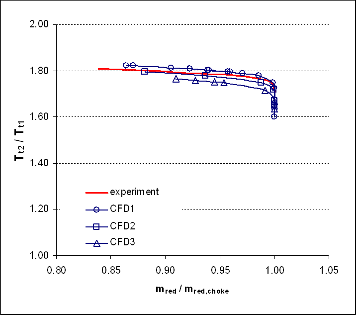
The total pressure ratio of CFD1, CFD2 and CFD3 is compared with the measured stage characteristic in Fig. 3.3. As to be expected the predicted maximum pressure ratio and operating range decrease with increased tip gap width. The measured peak pressure ratio lies between the result of CFD1 and CFD2, whereas the level of CFD3 is much too low.
All simulations show a 3.5-4% higher choke margin than the experiments, which is a direct consequence of the neglect of the blade hub fillet in the geometry. Therefore, for the following comparisons mred/mred,choke is used as the abscissa (instead of mred).

Fig 3.3 Total pressure rise for the stage (P04/P01)
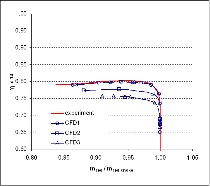
Isentropic efficiency and total pressure ratio for the rotor and the stator area presented in Fig. 3.4 and 3.5. While the isentropic efficiency for the rotor is over-estimated for all test cases, the agreement between the measured stage efficiency and CFD1 regarding the peak level as well as the shape of the characteristic is very good. The same is true for the total pressure rise.
It is worth noting here, that the interface between rotor and stator is not a mixing plane, but a so-called “frozen rotor” interface with no pitch change. This means the velocity components are merely converted from the rotating to the stationary frame of reference without any artificial mixing losses.
The fact that the agreement is worse for the rotor efficiency and the rotor total pressure rise is presumably caused by the way the measured total pressure at the rotor outlet was derived, i.e. from the measured total temperature, mass flow and the static pressure (at shroud) assuming a blocking factor of 17%. An increased blocking factor would lead to a higher total pressure ratio for the rotor. Because the correct value for the blocking factor is not known, it had to be taken from an initial CFD simulation. Therefore, the stage efficiency and stage total pressure rise seems to be more reliable, as the total pressure is explicitly measured at the exit.

Fig. 3.4 Isentropic efficiency for the impeller (η12) and the stage (η14)

Fig. 3.5 Total pressure ratio for the impeller (P02/P01) and the stage (P04/P01)
Available data files
• char1.dat measured characteristic
• char2.dat calculated characteristic (CFD1)
• char3.dat calculated characteristic (CFD2)
• char4.dat calculated characteristic (CFD3)
Available graphical comparisons
• char1.png comparison of rotor efficiency
• char2.png comparison of rotor total pressure ratio
• char3.png comparison of rotor total temperature ratio
• char4.png comparison of stage efficiency
• char5.png comparison of stage total pressure ratio
• char6.png comparison of stage total temperature ratio
© copyright ERCOFTAC 2004
Contributors: Beat Ribi; Frank Sieverding - MAN Turbomaschinen AG Schweiz; Sulzer Innotec AG