UFR 1-05 Test Case: Difference between revisions
m (Dave.Ellacott moved page Silver:UFR 1-05 Test Case to UFR 1-05 Test Case over redirect) |
|||
| (61 intermediate revisions by the same user not shown) | |||
| Line 81: | Line 81: | ||
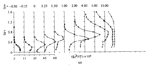
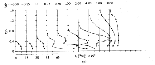
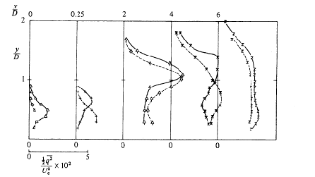
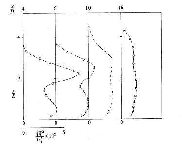
Profiles of turbulent kinetic energy, expressed as | Profiles of turbulent kinetic energy, expressed as | ||
for the three velocity ratios are also given. The authors distinguish three regions. The first one is over the exit of the jet, with various velocity gradients. The second one is immediately downstream, with a high production of turbulence due to the velocity gradient | <center><math> | ||
\frac{1}{2}\overline{q^2}=\frac{1}{2}\left(\overline{u^2}+\overline{v^2}+\overline{w^2}\right) | |||
</math></center> | |||
for the three velocity ratios are also given. The authors distinguish three regions. The first one is over the exit of the jet, with various velocity gradients. The second one is immediately downstream, with a high production of turbulence due to the velocity gradient | |||
<math>\partial U/\partial y</math>. | |||
In the third region the turbulent kinetic energy starts to decay as the mean velocity gradients become smaller. Profiles of turbulent kinetic energy for R=0.5, 1 and 2 are reproduced in Figs. 4.7, 4.8 and 4.9. | |||
| Line 110: | Line 116: | ||
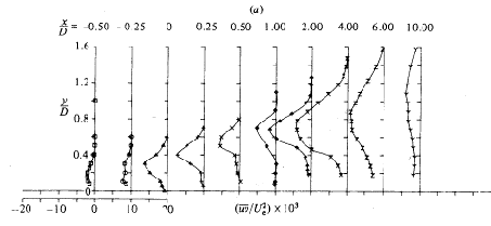
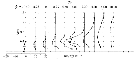
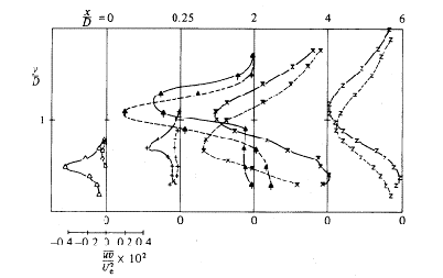
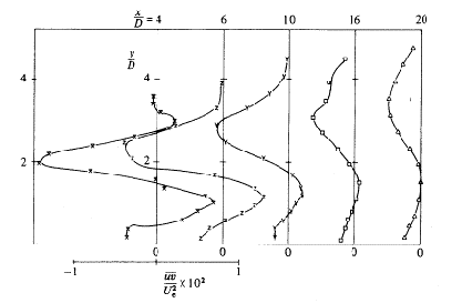
Finally, Andreopoulos and Rodi (1984) give the measurements of turbulent shear stresses for the same downstream and spanwise locations and velocity ratios for which the turbulent kinetic energy profiles were presented. Figures 4.10 to 4.12, copied from the authors, show the profiles. | Finally, Andreopoulos and Rodi (1984) give the measurements of turbulent shear stresses for the same downstream and spanwise locations and velocity ratios for which the turbulent kinetic energy profiles were presented. Figures 4.10 to 4.12, copied from the authors, show the profiles. | ||
The measurements have shown that in general the shear stress | The measurements have shown that in general the shear stress | ||
<math>\overline{uv}</math> | |||
can be described by an eddy viscosity model. However, in certain regions, this is not true because the shear stress | |||
<math>\overline{uv}</math> | |||
and the velocity gradient | |||
<math>\partial U/\partial y</math> | |||
have opposite signs (this would lead to negative eddy viscosity, compare Figs. 4.2 to 4.4 with Figs. 4.10 to 4.12) and | |||
<math>\partial W/\partial z</math> | |||
also contributes significantly to the production of | |||
<math>\overline{uv}</math>. | |||
The shear stress | |||
<math>\overline{uw}</math>, | |||
which controls the lateral spread of the jet, was found to be generated mainly by | |||
<math>\partial U/\partial z</math> | |||
and | |||
<math>\partial W/\partial y</math>. | |||
Since <math>\partial W/\partial y</math> | |||
does not appear in the eddy viscosity relation for | |||
<math>\overline{uw}</math>, | |||
this relation cannot describe | |||
<math>\overline{uw}</math> realistically. The shear stress | |||
<math>\overline{vw}</math>, | |||
which acts to damp the secondary vortex motion, was found to be closely related to the gradients | |||
<math>\partial V/\partial z</math> | |||
and <math>\partial W/\partial y</math> | |||
and so can probably be simulated in general with an eddy viscosity model. | |||
| Line 117: | Line 148: | ||
<center>[[Image:U1-05d32_files_image072.gif]]</center> | <center>[[Image:U1-05d32_files_image072.gif]]</center> | ||
<center>''Fig. 4.10 - < | <center>''Fig. 4.10 - ''<math>\overline{uv}</math> ''shear stress profiles for R=0.5; | ||
(a) Z/d=0 and (b) Z/d=0.5''</center> | |||
<center>Andreopoulos and Rodi (1984)</center> | <center>Andreopoulos and Rodi (1984)</center> | ||
| Line 123: | Line 155: | ||
<center>[[Image:U1-05d32_files_image076.gif]]</center> | <center>[[Image:U1-05d32_files_image076.gif]]</center> | ||
<center>''Fig. 4.11 - < | <center>''Fig. 4.11 - ''<math>\overline{uv}</math> ''shear stress profiles for R=1 – solid line z/D=0, dotted line z/D=-0.5''</center> | ||
<center>''Andreopoulos and Rodi (1984)''</center> | <center>''Andreopoulos and Rodi (1984)''</center> | ||
| Line 129: | Line 161: | ||
<center>[[Image:U1-05d32_files_image079.gif]]</center> | <center>[[Image:U1-05d32_files_image079.gif]]</center> | ||
<center>''Fig. 4.12 - < | <center>''Fig. 4.12 - ''<math>\overline{uv}</math> ''shear stress profiles for R=2 at Z/d=0''</center> | ||
<center>''Andreopoulos and Rodi (1984)''</center> | <center>''Andreopoulos and Rodi (1984)''</center> | ||
| Line 135: | Line 167: | ||
=== Measurements of the Flow & Turbulence Characteristics of Round Jets in Cross Flow – Sherif & Pletcher (1989) === | === Measurements of the Flow & Turbulence Characteristics of Round Jets in Cross Flow – Sherif & Pletcher (1989) === | ||
==== Objectives and Test Facility''' ==== | |||
Sherif & Pletcher (1989) measured velocity magnitudes in the streamline direction, streamwise and vertical components of velocity, overall turbulence intensity in the mean flow direction; turbulent stresses, structural parameter, correlation coefficient and the kinetic energy of turbulence. The measurements were carried out in the jet and in the wake, in and outside the jet plane of symmetry. Velocity ratios were 2, 4 and 6. | Sherif & Pletcher (1989) measured velocity magnitudes in the streamline direction, streamwise and vertical components of velocity, overall turbulence intensity in the mean flow direction; turbulent stresses, structural parameter, correlation coefficient and the kinetic energy of turbulence. The measurements were carried out in the jet and in the wake, in and outside the jet plane of symmetry. Velocity ratios were 2, 4 and 6. | ||
| Line 146: | Line 176: | ||
<center>[[Image:U1-05d32_files_image082.gif]]</center> | |||
<center>''Fig. 4.13 – Jet injection system''</center> | |||
[[Image:U1-05d32_files_image082.gif]] | |||
< | |||
<center>''Fig. 4.13 | |||
<center>''Sherif & Pletcher (1989)''</center> | <center>''Sherif & Pletcher (1989)''</center> | ||
| Line 165: | Line 183: | ||
==== Results ==== | |||
Unfortunately, due to the quality of the pictures in the paper, it would be useless to reproduce them here. The interested reader is encouraged to seek the original paper. | Unfortunately, due to the quality of the pictures in the paper, it would be useless to reproduce them here. The interested reader is encouraged to seek the original paper. | ||
| Line 179: | Line 197: | ||
<u>Structure of the velocity field</u> | <u>Structure of the velocity field</u> | ||
The rotational hot film probe technique used to measure the streamwise and vertical components of velocity is not capable to detect flow reversals. Maximum uncertainty is of 6% for | The rotational hot film probe technique used to measure the streamwise and vertical components of velocity is not capable to detect flow reversals. Maximum uncertainty is of 6% for | ||
<math>\overline{U}</math> and 7.5% for <math>\overline{W}</math>. | |||
The authors plot these components for an isothermal jet at a velocity ratio of 6, at locations x/D = 5.505 and 12.844 and at distances from the plane of symmetry y/D = 0, 0.115, 0.231, 0.347, 0.692 and 1.150. The streamwise component has an absolute maximum located in the jet field and a local maximum in the wake like region. The streamwise component becomes flatter, with less abrupt changes at x/D = 12.844 than at x/D = 5.505. | |||
The vertical component has an absolute maximum right below the location where the streamwise component reaches an absolute maximum, in the vertical direction. As z/D increases, the vertical component decreases non-linearly and is almost zero far above the jet. | The vertical component has an absolute maximum right below the location where the streamwise component reaches an absolute maximum, in the vertical direction. As z/D increases, the vertical component decreases non-linearly and is almost zero far above the jet. | ||
| Line 197: | Line 217: | ||
The correlation coefficient [[Image:U1-05d32_files_image096.gif]] describes the development of the Reynolds shear stress relative to the product of the streamwise and vertical components of the turbulent velocity fluctuations. It is presented at the same positions and the same velocity ratio for which the structural parameter was shown, with uncertainty 17%. The maximum value increases from about 0.7 in the jet plane of symmetry to about 1.0 at y/D=1.150. Locations of the peaks are the same as those of the structural parameter, where the shear stress is a maximum. | The correlation coefficient [[Image:U1-05d32_files_image096.gif]] describes the development of the Reynolds shear stress relative to the product of the streamwise and vertical components of the turbulent velocity fluctuations. It is presented at the same positions and the same velocity ratio for which the structural parameter was shown, with uncertainty 17%. The maximum value increases from about 0.7 in the jet plane of symmetry to about 1.0 at y/D=1.150. Locations of the peaks are the same as those of the structural parameter, where the shear stress is a maximum. | ||
=== Effects of Swirl and High Turbulence on a Jet in Cross Flow – Kavsaoglu and Schetz (1989) === | |||
==== Objectives and Test Facility ==== | |||
Kavsaoglu and Schetz (1989) studied the effects of different jet exit velocity profiles and jet exit turbulence levels on a jet in cross flow. They considered a circular jet hitting the main flow at 90 degrees. Jet types were 1) low turbulence (3%), uniform profile, 2) high turbulence (>10%), uniform profile, and 3) swirling. Swirl ratios of 40% and 58% were studied (maximum peripheral velocity over average axial velocity). Surface pressure distributions were obtained for R=2.2, 4 and 8. High turbulence was not studied with R=8. Mean velocities were obtained for R=4. Turbulence intensities and Reynolds stresses were measured for R=4. | Kavsaoglu and Schetz (1989) studied the effects of different jet exit velocity profiles and jet exit turbulence levels on a jet in cross flow. They considered a circular jet hitting the main flow at 90 degrees. Jet types were 1) low turbulence (3%), uniform profile, 2) high turbulence (>10%), uniform profile, and 3) swirling. Swirl ratios of 40% and 58% were studied (maximum peripheral velocity over average axial velocity). Surface pressure distributions were obtained for R=2.2, 4 and 8. High turbulence was not studied with R=8. Mean velocities were obtained for R=4. Turbulence intensities and Reynolds stresses were measured for R=4. | ||
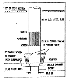
Figure 4.14 schematically shows the Stability Tunnel used at Virginia Polytechnic Institute. The jet was injected from a 1.78m x 2.13m flat plate. The jet diameter was 49.2 mm and it was exhausted downwards at 48.3 cm behind the leading edge. An area of 30.48 cm x 40.64 cm was covered with more than 450 pressure taps. Air passed through a 8.6 cm diam steel tube 50 cm long. At the end of this tube, a pair of 1.59 cm copper tubes were connected for tangential air injection to produce swirl. The steel tube was followed by a 2.38 cm long contraction and a 3 cm long, 49.2 mm diam constant area section before the jet exit. For high turbulence experiments, a turbulence generating screen was placed right after the contraction. | |||
<center>[[Image:U1-05d32_files_image102.gif]]</center> | |||
<center>''Fig. 4.14 – Jet nozzle assembly – Kavsaoglu and Schetz (1989)''</center> | |||
==== Results ==== | |||
Pressure distribution results are given as pressure coefficients, expressed by | Pressure distribution results are given as pressure coefficients, expressed by | ||
<math>\Delta C_p=\left(C_{p,\ \mathrm{jet\_on}}-C_{p,\ \mathrm{jet\_off}}\right)</math> | |||
where <math>C_p=(p-p_\infty)/q_\infty</math>, | |||
p = static pressure and q = dynamic pressure | <math>p</math> = static pressure and <math>q</math> = dynamic pressure. | ||
A negative pressure region extending to the lateral and downstream directions was found. The magnitudes at the left and right sides of the jet were about | A negative pressure region extending to the lateral and downstream directions was found. The magnitudes at the left and right sides of the jet were about -3, -5 and -4 for R=2.2, 4 and 8 respectively. The authors noticed that, for high turbulence jet (10% in the centre and >16% at the periphery), the negative pressure area was smaller than for low turbulence, though the magnitude of negative pressures did not change for R=2.2 and R=4. Increasing exit turbulence also produced more symmetric pressure distributions. | ||
With jet with swirl and R=2.2, a strongly asymmetric pressure distribution was observed. However, with R=4 and 8, the asymmetric pressure distribution due to swirl cannot be observed any more for the 40% swirl case. It was observed that in general swirl has more influence for the low velocity ratios and on the area close to the jet exit. | With jet with swirl and R=2.2, a strongly asymmetric pressure distribution was observed. However, with R=4 and 8, the asymmetric pressure distribution due to swirl cannot be observed any more for the 40% swirl case. It was observed that in general swirl has more influence for the low velocity ratios and on the area close to the jet exit. | ||
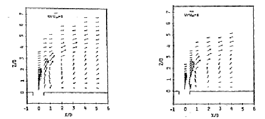
Mean velocities for R=4 are reproduced in Figs. 4.15 to 4.18. Around x/D = 6 (x = direction of the main stream), most of the downstream turning of the jet has occurred. The authors define | Mean velocities for R=4 are reproduced in Figs. 4.15 to 4.18. Around x/D = 6 (x = direction of the main stream), most of the downstream turning of the jet has occurred. The authors define ‘penetration height’ the height of the jet center at this point. In Figs. 4.15 to 4.17, the results for the jet center plane (y/D=0) can be seen for the low turbulence jet, high turbulence jet and 58% swirl jet. The authors found that the penetration height was 30% smaller in the high turbulence, 58% swirl case, than in the low turbulence, no swirl case. This is a very important result for blade cooling, as the designer would like the jet to be as close to the blade surface as possible, with minimal mixing into the main stream. | ||
< | <center>[[Image:U1-05d32_files_image104.gif]]</center> | ||
<center>''Fig. 4.15 – Low turbulence, R=4, x/D=6 Fig. 4.16 – High turbulence, R=4, x/D=6''</center> | |||
< | <center>[[Image:U1-05d32_files_image106.gif]]</center> | ||
<center>'' Fig. 4.17 – 58% swirl jet, R=4, x/D=6 Fig. 4.18 – 58% swirl jet, R=4, x/D=1.026''</center> | |||
== CFD Methods == | |||
=== Large Eddy Simulations of a Round Jet in Cross Flow – Yuan, Street and Ferziger (1999) === | |||
==== Previous work on turbulence models in JICF ==== | |||
Yuan et al. (1999) describe the attempts made by several authors to model the jet in cross flow, using different turbulence modelling techniques. Sykes et al. (1986) solved the jet in cross flow using a version of the Mellor Yamada 2.5 turbulence model. They used a limited number of points and did not resolve the flow near the bottom wall. Claus and Vanka (1992) used a simple [[Image:U1-05d32_files_image108.gif]] turbulence model with many more points and still had trouble reproducing mean experimental results and concluded from their study that Reynolds-averaged Navier-Stokes models developed for use with simple boundary layer flows were not accurate enough for the complexities of the jet in cross flow. This is in agreement with the conclusions of Andreopoulos and Rodi (1984). Kim and Benson (1992) attempted to improve the turbulence model introducing turbulent time scales which vary in the flow and introduced a better modelling of the jet inflow boundary condition, reproducing the flow statistics well but not the turbulent kinetic energy. Demuren (1993) modelled the full Reynolds stress transport equations but failed to accurately reproduce the mean velocities and the turbulent kinetic energy. Yuan et al. (1999) also refer to time-accurate simulations made by Rudman (1994) and Jones & Wille (1996). Inaccuracies have been found, due to lack of adequate resolution of the scales of motion and to not considering the turbulent wall boundary layer. | |||
==== Large-eddy simulations — equations and numerical method ==== | |||
Yuan et al. (1999) report on large-eddy simulations of the jet in cross flow. They solved the grid-filtered incompressible Navier-Stokes equations: | |||
<center><math>\frac{\partial\ \overline{u_k}}{\partial x_k}=0</math></center> | |||
<center><math> | |||
\frac{\partial\ \overline{u_i}}{\partial t}+\frac{\partial}{\partial x_j}\left(\overline{u_j} | |||
\ \overline{u_i}\right)=-\frac{\partial\ \overline{p}}{\partial x_i}+\frac{1}{{Re}_D} | |||
\frac{\partial^2\overline{u_i}}{\partial x_j^2}-\frac{\partial}{\partial x_j}\tau_{ij} | |||
</math></center> | |||
where a line over a variable indicates a grid-filtered quantity; | |||
<math>u_i</math> are the Cartesian velocity components non-dimensionalized by the cross flow velocity | |||
<math>U_\infty^2</math> | |||
and the spatial coordinates are non-dimensionalized by the jet diameter <math>D</math>. | |||
The Reynolds number is defined as | |||
<center><math>{Re}_D=\frac{U_\infty D}{\nu}</math></center> | |||
where | where the kinematic viscosity <math>\left.\nu\right.</math> is assumed constant. | ||
Effects of velocities not resolved by the computational grid are included through a sub-grid scale stress defined as | |||
<center><math>\tau_{ij}=\overline{u_i u_j}-\overline{u_i}\ \overline{u_j}</math></center> | |||
To model this stress a dynamic subgrid-scale model is used (Zang, Streeet and Koseff (1993)), known to be effective in transitionally turbulent flows and stable. The governing equations are solved with a control volume formulation in a generalized coordinate system, using a fractional step, non-staggered solution technique of Zang, Street and Koseff (1994). Two sets of variables are used, defining Cartesian velocities and pressures at cell centres and contravariant volume fluxes at cell faces. The solution is advanced in time with a semi-implicit, second-order accurate scheme. Spatial discretization is also second-order accurate. About the code, the authors say that grid resolution studies showed that while some minor quantitative changes occur as the grids are refined, the code reproduces the same qualitative features as long as the large scale structures are resolved. In the simulation of the jet in cross flow, thirteen grids were used to resolve the circular boundary condition of the jet exit and the flow through the main channel. This domain decomposition is made according to techniques given by Zang & Street (1995). | To model this stress a dynamic subgrid-scale model is used (Zang, Streeet and Koseff (1993)), known to be effective in transitionally turbulent flows and stable. The governing equations are solved with a control volume formulation in a generalized coordinate system, using a fractional step, non-staggered solution technique of Zang, Street and Koseff (1994). Two sets of variables are used, defining Cartesian velocities and pressures at cell centres and contravariant volume fluxes at cell faces. The solution is advanced in time with a semi-implicit, second-order accurate scheme. Spatial discretization is also second-order accurate. About the code, the authors say that grid resolution studies showed that while some minor quantitative changes occur as the grids are refined, the code reproduces the same qualitative features as long as the large scale structures are resolved. In the simulation of the jet in cross flow, thirteen grids were used to resolve the circular boundary condition of the jet exit and the flow through the main channel. This domain decomposition is made according to techniques given by Zang & Street (1995). | ||
| Line 306: | Line 304: | ||
<center>[[Image:U1-05d32_files_image124.gif]]</center> | |||
<center>''Fig. 5.1 – Flow configuration – adapted from Yuan et al. (1999)''</center> | |||
[[Image:U1-05d32_files_image124.gif]] | |||
<center>''Fig. 5.1 | |||
| Line 325: | Line 313: | ||
For stability, the fine grids and high velocities led to very small simulation time steps. In consequence, each simulation required approximately 2000 hours on a single processor Cray J90 and approximately 500 hours on a single processor of a Cray C90. The computer time can be evaluated as given by 80 T<sub>u</sub>= 80 ''D/U<sub>∞</sub>''. | For stability, the fine grids and high velocities led to very small simulation time steps. In consequence, each simulation required approximately 2000 hours on a single processor Cray J90 and approximately 500 hours on a single processor of a Cray C90. The computer time can be evaluated as given by 80 T<sub>u</sub>= 80 ''D/U<sub>∞</sub>''. | ||
==== Comparisons to experiment ==== | |||
Yuan et al. (1999) made the computations for 3 different cases, to compare results with the experimental data given by Sherif & Pletcher (1989, some times referred to below as SP), with jet radius and Reynolds numbers at the pipe as shown in Table 5.1. | Yuan et al. (1999) made the computations for 3 different cases, to compare results with the experimental data given by Sherif & Pletcher (1989, some times referred to below as SP), with jet radius and Reynolds numbers at the pipe as shown in Table 5.1. | ||
| Line 372: | Line 358: | ||
Quantities in the centre plane were calculated by Yuan et al (1999) by using the equations: | Quantities in the centre plane were calculated by Yuan et al (1999) by using the equations: | ||
<center><math>U_m=\left(u_1^2+u_2^2+u_3^2\right)^{1/2}</math></center> | |||
<center><math>u_m^\mathrm{ff}=U_m-\langle U_m\rangle</math></center> | |||
<center><math>u_\mathrm{rms}=\langle u_m^\mathrm{ff}\rangle^{1/2}</math></center> | |||
where [[Image:U1-05d32_files_image132.gif]] denotes long time average. | |||
Fig. 5.2 shows vertical profiles of velocity magnitude on the centreplane at four streamwise locations, for cases 3I and 3II. Case 3II profiles seem to match experiment closely, above the point of maximum velocity. Below this point the velocity magnitudes are higher than experiment. | |||
<center>[[Image:U1-05d32_files_image134.gif]]</center> | |||
<center>''Fig. 5.2 – Vertical profiles of mean velocity magnitude at the centre-plane.</center> | |||
<center>Solid line, Case 3II; dashed line, Case 3I; open circles, SP.''</center> | |||
<center> | <center>[[Image:U1-05d32_files_image136.gif]]</center> | ||
<center>''Fig. 5.3 – Vertical profiles of r.m.s. fluctuations in velocity magnitude.''</center> | |||
<center>''Solid line: Case 3II; dashed line: Case 3I; open circles: SP.''</center> | <center>''Solid line: Case 3II; dashed line: Case 3I; open circles: SP.''</center> | ||
In Fig. 5.3 the authors plot the r.m.s. fluctuations of velocity magnitude defined in | In Fig. 5.3 the authors plot the r.m.s. fluctuations of velocity magnitude defined in the above equations for cases 3I and 3II against the experimental measurements of Sherif & Pletcher. Case 3II compares better with experiment. However, although over the jet exit the agreement between Case 3II and experiment is excellent, at stations downstream r.m.s. magnitudes are underpredicted in the lower half of the profile. A second peak that appears near the wall, particularly at x=1.84 and x=5.54, is explained by fluctuations generated by the wall wake vortices. Through some calculations based on boundary layer theory, the authors show that the higher velocities observed in the lower portions of the velocity profiles are due to differences between the flat plate boundary layers in the simulations and the experiments. | ||
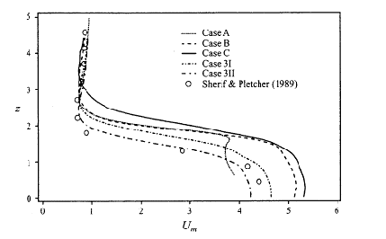
It has been found, both experimentally and computationally that the development of the downstream flow is particularly sensitive to the characteristics of the inflow jet. Different types of inflow conditions have been tried by the authors in cases A, B and C, where they varied the velocity ratio R and the flow condition (Table 5.2). | It has been found, both experimentally and computationally that the development of the downstream flow is particularly sensitive to the characteristics of the inflow jet. Different types of inflow conditions have been tried by the authors in cases A, B and C, where they varied the velocity ratio R and the flow condition (Table 5.2). | ||
| Line 484: | Line 455: | ||
<center>[[Image:U1-05d32_files_image138.gif]]</center> | |||
<center>''Fig. 5.4 – Effect of jet inflow conditions''</center> | |||
[[Image:U1-05d32_files_image138.gif]] | |||
< | |||
<center>''Fig. 5.4 | |||
<center>''Solid line, Case 3II; dashed line, case 3I; open circles, SP.''</center> | <center>''Solid line, Case 3II; dashed line, case 3I; open circles, SP.''</center> | ||
| Line 506: | Line 465: | ||
Given the uncertainties in the experiments, particularly with respect to the boundary layer and to the pipe flow, the agreement between calculations and experiments is very good. | Given the uncertainties in the experiments, particularly with respect to the boundary layer and to the pipe flow, the agreement between calculations and experiments is very good. | ||
=== Navier-Stokes Analysis of a Swirling Jet in a Cross Flow – Yagci and Kavsaoglu (1993) === | |||
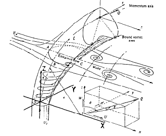
Yagci and Kavsaoglu (1993) analysed a swirling subsonic jet injected into a subsonic cross flow, using a three dimensional, thin layer, Reynolds averaged, compressible Navier Stokes solver. The flow and the coordinate system are described in Fig. 5.5, reproduced from the authors. | Yagci and Kavsaoglu (1993) analysed a swirling subsonic jet injected into a subsonic cross flow, using a three dimensional, thin layer, Reynolds averaged, compressible Navier Stokes solver. The flow and the coordinate system are described in Fig. 5.5, reproduced from the authors. | ||
| Line 514: | Line 471: | ||
In the jet region they used the algebraic turbulence model proposed by Oh and Schetz (1990). In other viscous turbulent flow areas they used the Baldwin Lomax turbulence model. Riemann invariants based characteristic boundary conditions have been considered as input boundary conditions for the main flow. At the output they used inverse characteristic boundary conditions. Their test case is the experimental case with 58% swirl, with velocity ratio 4, as described by Kavsaoglu and Schetz (1989). | In the jet region they used the algebraic turbulence model proposed by Oh and Schetz (1990). In other viscous turbulent flow areas they used the Baldwin Lomax turbulence model. Riemann invariants based characteristic boundary conditions have been considered as input boundary conditions for the main flow. At the output they used inverse characteristic boundary conditions. Their test case is the experimental case with 58% swirl, with velocity ratio 4, as described by Kavsaoglu and Schetz (1989). | ||
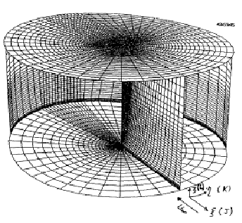
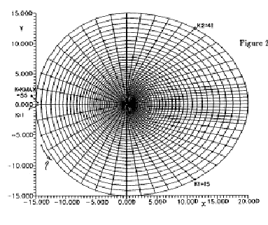
Their grid was obtained by rotation of a two dimensional half grid around the jet axis. The grid had a cavity at the jet entrance. This grid was extended from | Their grid was obtained by rotation of a two dimensional half grid around the jet axis. The grid had a cavity at the jet entrance. This grid was extended from -15 D to 20 D in the x direction, from -15 D to 15 D in the y direction and from -0.5 D to 15 D in the z direction where D is the jet exit diameter. The size of the grid was 42 x 55 x 45 points, in the x, h, z directions (Figs. 5.6 to 5.8). | ||
<center>[[Image:U1-05d32_files_image140.gif]]</center> | |||
<center>''Fig. 5.5 – Flow field description of a round jet in a cross flow''</center> | |||
[[Image:U1-05d32_files_image140.gif]] | |||
<center>''Fig. 5.5 | |||
<center>''Yagci & Kavsaoglu (1993)''</center> | <center>''Yagci & Kavsaoglu (1993)''</center> | ||
| Line 538: | Line 485: | ||
<center>[[Image:U1-05d32_files_image142.gif]]</center> | |||
<center>''Fig. 5.6 – Three dimensional view of the grid. ''</center> | |||
[[Image:U1-05d32_files_image142.gif]] | |||
< | |||
<center>''Fig. 5.6 | |||
<center>''Yagci and Kavsaoglu (1993)''</center> | <center>''Yagci and Kavsaoglu (1993)''</center> | ||
<center>[[Image:U1-05d32_files_image144.gif]]</center> | |||
<center>''Fig. 5.7 – Top view of the grid.''</center> | |||
[[Image:U1-05d32_files_image144.gif]] | |||
< | |||
<center>''Fig. 5.7 | |||
<center>''Yagci and Kavsaoglu (1993)''</center> | <center>''Yagci and Kavsaoglu (1993)''</center> | ||
<center>[[Image:U1-05d32_files_image146.gif]]</center> | |||
<center>''Fig. 5.8 – Two dimensional section view of the grid around the cavity.''</center> | |||
[[Image:U1-05d32_files_image146.gif]] | |||
<center>''Fig. 5.8 | |||
<center>''Yagci and Kavsaoglu (1993)''</center> | <center>''Yagci and Kavsaoglu (1993)''</center> | ||
Latest revision as of 19:07, 11 February 2017
Jet in a cross flow
Underlying Flow Regime 1-05 © copyright ERCOFTAC 2004
Test Case
Brief description of the study test case
The study test cases generally involve a wind tunnel where a flat plate controls the development of a boundary layer. A pipe is adapted to the flat plate and a jet from the pipe hits the cross flow. The facilities used are shown in sketches below. Particularly important to define the experiments is the velocity ratio R = jet velocity / cross flow velocity. Also an important aspect to consider is whether the flow in the pipe is well developed when the jet leaves the pipe, because the boundary conditions to the CFD calculations must be consistent with the true velocity profile at the pipe exit in the experiments. Velocity field, particularly velocity components at the central plane of the jet, and turbulence parameters are the experimental quantities available for CFD validation. The following sections describe these data in detail.
Test Case Experiments
Experimental Investigation of Jets in Cross Flow — Andreopoulos and Rodi (1984)
Objectives and Test Facility
According to Andreopoulos and Rodi (1984), it is established that, at high velocity ratios, the near field of jets in cross flow is largely controlled by inviscid dynamics and so the influence of turbulence is limited. However, the flow further downstream is influenced by turbulence and, at low velocity ratios, even the near field is influenced by turbulence. The authors argue that previous measurements of turbulence data were either incomplete or inaccurate, for reasons they explain. The objective of their research programme was to increase understanding of the mean flow and turbulence characteristics of jets in a cross-stream at various velocity ratios and to obtain reliable and comprehensive turbulence data which can be used for testing and improving turbulence models. Their report presents measurements of mean and fluctuating velocities in the jet in a cross stream interaction region for velocity ratios R=0.5, 1 and 2. Triple-wire probes were used to capture the instantaneous values of the velocity vector. Description of the technique is detailed in their paper. The test facility is shown in Fig. 4.1.
The measurements of mean and fluctuating velocities for the three velocity ratios R=0.5, 1 and 2 were obtained by varying the velocity at the pipe and keeping the cross flow velocity constant at 13.9 m/s. Reynolds numbers based on the pipe diameter and jet velocity were 20500, 41000 and 82000. Turbulent flows were found for all velocity ratios investigated. Mean velocity profiles at various downstream positions are presented in the paper for the three velocity ratios and further profiles are available through a departmental report from the university.
Results
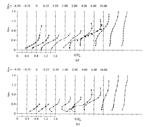
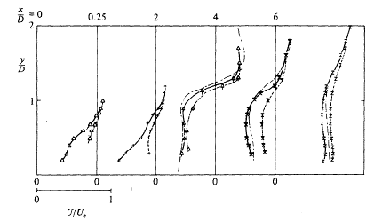
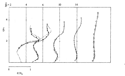
A sample of their results is reproduced here. The graphs in Figs. 4.2 to 4.4 show the profiles of the U velocity (x direction), divided by the cross stream velocity Ue, at the plane of symmetry and at the plane z/D = -0.5, at several x positions, for R=0.5, 1 and 2. Comparison with measurements made by other authors is also shown. Similar graphs are presented by the authors for the V and W components of velocity.

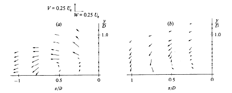
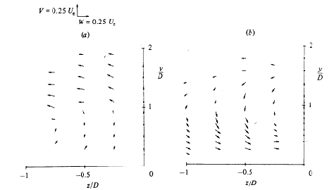
They also show (Figs. 4.5 and 4.6) secondary-motion velocity vectors. These graphs show the structure of the vortices and how the flow develops downstream the jet. For x/D=1, the vectors clearly show the upward and outward deflection of the cross flow by the bent-over jet and the formation of a vortex with anti-clockwise rotation. For x/D=2, the vectors show the superposition of the downward motion of the jet on the vortex. The reader should note that the fluid is moving towards the observer, out of the page, and that the plane of symmetry contains the axis y/D.
Profiles of turbulent kinetic energy, expressed as
for the three velocity ratios are also given. The authors distinguish three regions. The first one is over the exit of the jet, with various velocity gradients. The second one is immediately downstream, with a high production of turbulence due to the velocity gradient
.
In the third region the turbulent kinetic energy starts to decay as the mean velocity gradients become smaller. Profiles of turbulent kinetic energy for R=0.5, 1 and 2 are reproduced in Figs. 4.7, 4.8 and 4.9.
Finally, Andreopoulos and Rodi (1984) give the measurements of turbulent shear stresses for the same downstream and spanwise locations and velocity ratios for which the turbulent kinetic energy profiles were presented. Figures 4.10 to 4.12, copied from the authors, show the profiles.
The measurements have shown that in general the shear stress can be described by an eddy viscosity model. However, in certain regions, this is not true because the shear stress and the velocity gradient have opposite signs (this would lead to negative eddy viscosity, compare Figs. 4.2 to 4.4 with Figs. 4.10 to 4.12) and also contributes significantly to the production of . The shear stress , which controls the lateral spread of the jet, was found to be generated mainly by and . Since does not appear in the eddy viscosity relation for , this relation cannot describe realistically. The shear stress , which acts to damp the secondary vortex motion, was found to be closely related to the gradients and and so can probably be simulated in general with an eddy viscosity model.
Measurements of the Flow & Turbulence Characteristics of Round Jets in Cross Flow – Sherif & Pletcher (1989)
Objectives and Test Facility
Sherif & Pletcher (1989) measured velocity magnitudes in the streamline direction, streamwise and vertical components of velocity, overall turbulence intensity in the mean flow direction; turbulent stresses, structural parameter, correlation coefficient and the kinetic energy of turbulence. The measurements were carried out in the jet and in the wake, in and outside the jet plane of symmetry. Velocity ratios were 2, 4 and 6.
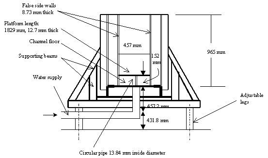
The equipment was a semiclosed circuit water channel at Iowa State University. The channel is 8.53 m long and 0.61 m x 1.067 m in cross section. Water circulated from an inlet tank through a transition section (area contraction approx. 5.25:1) to the tank, then to a pump and to the inlet tank. Some features were added to guarantee uniform stream velocity and low level of turbulence. Probes were positioned in three directions, controlled manually or by computer. Thermal anemometry was used. Normal and 45 degrees fiber film probes were used with anemometers operated in the constant temperature mode.
The plate length was chosen taking into account the range of jet trajectories for different jet inlet conditions. The plate width was chosen to avoid interference with the turbulent boundary layers already developed on the channel sides. The centre of the pipe was located 0.457 m downstream of the leading edge. Two false sidewalls were installed on both sides of the plate to promote two-dimensionality for the flow and to serve as supporting members for the plate.
Results
Unfortunately, due to the quality of the pictures in the paper, it would be useless to reproduce them here. The interested reader is encouraged to seek the original paper.
Mean velocity
Mean velocity profiles are given for velocity ratios 4 and 6. The absolute maximum of the mean velocity was found on the jet centre line trajectory for both velocity ratios. Its location depends upon the velocity ratio. Constant velocity contours are given at a number of stations downstream the jet.
Turbulence intensity
The authors found that above the jet discharge, where x/D=0, high turbulence intensity occurs at the interaction of the jet with the cross stream, where the velocity gradients are maximum. At x/D=1.835, the kidney-shaped region is a region of very high turbulence. At a turbulence intensity of 25%, the uncertainty in the turbulence reading was 2.5%. At 50% intensity it was 10%. At a given station x/D, the maximum turbulence intensity was observed to decrease with increasing velocity ratio. The authors mention that Madni (1975) found it necessary to include a velocity ratio parameter in the equation for the turbulent viscosity that decreases its value at larger velocity ratios.
Structure of the velocity field
The rotational hot film probe technique used to measure the streamwise and vertical components of velocity is not capable to detect flow reversals. Maximum uncertainty is of 6% for and 7.5% for . The authors plot these components for an isothermal jet at a velocity ratio of 6, at locations x/D = 5.505 and 12.844 and at distances from the plane of symmetry y/D = 0, 0.115, 0.231, 0.347, 0.692 and 1.150. The streamwise component has an absolute maximum located in the jet field and a local maximum in the wake like region. The streamwise component becomes flatter, with less abrupt changes at x/D = 12.844 than at x/D = 5.505.
The vertical component has an absolute maximum right below the location where the streamwise component reaches an absolute maximum, in the vertical direction. As z/D increases, the vertical component decreases non-linearly and is almost zero far above the jet.
Kinetic energy of turbulence
The authors give profiles of kinetic energy of turbulence ![]() for an isothermal jet at a velocity ratio of 4, discharge Reynolds number of 18036 and stations x/D = 5.505 and 12.844 and transverse positions y/D = 0, 0.115, 0.231, 0.347, 0.692 and 1.150, with maximum uncertainty estimated in 7%.
for an isothermal jet at a velocity ratio of 4, discharge Reynolds number of 18036 and stations x/D = 5.505 and 12.844 and transverse positions y/D = 0, 0.115, 0.231, 0.347, 0.692 and 1.150, with maximum uncertainty estimated in 7%.
At x/D = 5.505, the profiles are nearly the same up to a transverse position y/D = 0.692. The turbulent kinetic energy has an absolute maximum and a local maximum similar to the mean velocity profiles. The location of the absolute maximum outside the plane of symmetry up to y/D = 0.692 corresponds very closely to that in the plane of symmetry. Andreopoulos and Rodi (1984) found the same for velocity ratio 2. The double peak in the ![]() profiles, found by Andreopoulos and Rodi (1984) to be hardly noticeable for velocity ratio R=0.5 and increasingly significant for R=1 and R=2, was found by Sherif and Pletcher still more significant for R=4.
profiles, found by Andreopoulos and Rodi (1984) to be hardly noticeable for velocity ratio R=0.5 and increasingly significant for R=1 and R=2, was found by Sherif and Pletcher still more significant for R=4.
Reynolds Stress, Structural Parameter and Correlation Coefficient
Profiles of the Reynolds stress parameter ![]() are presented for the same isothermal jet for x/D = 12.844 and the same spanwise locations where turbulent kinetic energy profiles are presented, with measurement uncertainty 8%. With increasing transverse distance, the shear stress increases and the location at which the maximum shear stress occurs moves farther from the wall. The structural parameter
are presented for the same isothermal jet for x/D = 12.844 and the same spanwise locations where turbulent kinetic energy profiles are presented, with measurement uncertainty 8%. With increasing transverse distance, the shear stress increases and the location at which the maximum shear stress occurs moves farther from the wall. The structural parameter ![]() is presented for the same jet at the same streamwise and spanwise positions, with uncertainty 14%. The authors found the maximum value of the structural parameter was 0.59, at x/D = 10 and y/D = 1.150. In the plane of symmetry the peak value was 0.48. At x/D close to 10, Andreopulos and Rodi (1984) found the maximum value of the structural parameter equal to 0.30, with R=0.5, much lower than the value found by the authors. They argue this may be due to different flow character, caused by different R values.
is presented for the same jet at the same streamwise and spanwise positions, with uncertainty 14%. The authors found the maximum value of the structural parameter was 0.59, at x/D = 10 and y/D = 1.150. In the plane of symmetry the peak value was 0.48. At x/D close to 10, Andreopulos and Rodi (1984) found the maximum value of the structural parameter equal to 0.30, with R=0.5, much lower than the value found by the authors. They argue this may be due to different flow character, caused by different R values.
Correlation coefficient
The correlation coefficient ![]() describes the development of the Reynolds shear stress relative to the product of the streamwise and vertical components of the turbulent velocity fluctuations. It is presented at the same positions and the same velocity ratio for which the structural parameter was shown, with uncertainty 17%. The maximum value increases from about 0.7 in the jet plane of symmetry to about 1.0 at y/D=1.150. Locations of the peaks are the same as those of the structural parameter, where the shear stress is a maximum.
describes the development of the Reynolds shear stress relative to the product of the streamwise and vertical components of the turbulent velocity fluctuations. It is presented at the same positions and the same velocity ratio for which the structural parameter was shown, with uncertainty 17%. The maximum value increases from about 0.7 in the jet plane of symmetry to about 1.0 at y/D=1.150. Locations of the peaks are the same as those of the structural parameter, where the shear stress is a maximum.
Effects of Swirl and High Turbulence on a Jet in Cross Flow – Kavsaoglu and Schetz (1989)
Objectives and Test Facility
Kavsaoglu and Schetz (1989) studied the effects of different jet exit velocity profiles and jet exit turbulence levels on a jet in cross flow. They considered a circular jet hitting the main flow at 90 degrees. Jet types were 1) low turbulence (3%), uniform profile, 2) high turbulence (>10%), uniform profile, and 3) swirling. Swirl ratios of 40% and 58% were studied (maximum peripheral velocity over average axial velocity). Surface pressure distributions were obtained for R=2.2, 4 and 8. High turbulence was not studied with R=8. Mean velocities were obtained for R=4. Turbulence intensities and Reynolds stresses were measured for R=4.
Figure 4.14 schematically shows the Stability Tunnel used at Virginia Polytechnic Institute. The jet was injected from a 1.78m x 2.13m flat plate. The jet diameter was 49.2 mm and it was exhausted downwards at 48.3 cm behind the leading edge. An area of 30.48 cm x 40.64 cm was covered with more than 450 pressure taps. Air passed through a 8.6 cm diam steel tube 50 cm long. At the end of this tube, a pair of 1.59 cm copper tubes were connected for tangential air injection to produce swirl. The steel tube was followed by a 2.38 cm long contraction and a 3 cm long, 49.2 mm diam constant area section before the jet exit. For high turbulence experiments, a turbulence generating screen was placed right after the contraction.
Results
Pressure distribution results are given as pressure coefficients, expressed by
where ,
= static pressure and = dynamic pressure.
A negative pressure region extending to the lateral and downstream directions was found. The magnitudes at the left and right sides of the jet were about -3, -5 and -4 for R=2.2, 4 and 8 respectively. The authors noticed that, for high turbulence jet (10% in the centre and >16% at the periphery), the negative pressure area was smaller than for low turbulence, though the magnitude of negative pressures did not change for R=2.2 and R=4. Increasing exit turbulence also produced more symmetric pressure distributions.
With jet with swirl and R=2.2, a strongly asymmetric pressure distribution was observed. However, with R=4 and 8, the asymmetric pressure distribution due to swirl cannot be observed any more for the 40% swirl case. It was observed that in general swirl has more influence for the low velocity ratios and on the area close to the jet exit.
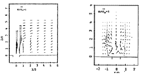
Mean velocities for R=4 are reproduced in Figs. 4.15 to 4.18. Around x/D = 6 (x = direction of the main stream), most of the downstream turning of the jet has occurred. The authors define ‘penetration height’ the height of the jet center at this point. In Figs. 4.15 to 4.17, the results for the jet center plane (y/D=0) can be seen for the low turbulence jet, high turbulence jet and 58% swirl jet. The authors found that the penetration height was 30% smaller in the high turbulence, 58% swirl case, than in the low turbulence, no swirl case. This is a very important result for blade cooling, as the designer would like the jet to be as close to the blade surface as possible, with minimal mixing into the main stream.
CFD Methods
Large Eddy Simulations of a Round Jet in Cross Flow – Yuan, Street and Ferziger (1999)
Previous work on turbulence models in JICF
Yuan et al. (1999) describe the attempts made by several authors to model the jet in cross flow, using different turbulence modelling techniques. Sykes et al. (1986) solved the jet in cross flow using a version of the Mellor Yamada 2.5 turbulence model. They used a limited number of points and did not resolve the flow near the bottom wall. Claus and Vanka (1992) used a simple ![]() turbulence model with many more points and still had trouble reproducing mean experimental results and concluded from their study that Reynolds-averaged Navier-Stokes models developed for use with simple boundary layer flows were not accurate enough for the complexities of the jet in cross flow. This is in agreement with the conclusions of Andreopoulos and Rodi (1984). Kim and Benson (1992) attempted to improve the turbulence model introducing turbulent time scales which vary in the flow and introduced a better modelling of the jet inflow boundary condition, reproducing the flow statistics well but not the turbulent kinetic energy. Demuren (1993) modelled the full Reynolds stress transport equations but failed to accurately reproduce the mean velocities and the turbulent kinetic energy. Yuan et al. (1999) also refer to time-accurate simulations made by Rudman (1994) and Jones & Wille (1996). Inaccuracies have been found, due to lack of adequate resolution of the scales of motion and to not considering the turbulent wall boundary layer.
turbulence model with many more points and still had trouble reproducing mean experimental results and concluded from their study that Reynolds-averaged Navier-Stokes models developed for use with simple boundary layer flows were not accurate enough for the complexities of the jet in cross flow. This is in agreement with the conclusions of Andreopoulos and Rodi (1984). Kim and Benson (1992) attempted to improve the turbulence model introducing turbulent time scales which vary in the flow and introduced a better modelling of the jet inflow boundary condition, reproducing the flow statistics well but not the turbulent kinetic energy. Demuren (1993) modelled the full Reynolds stress transport equations but failed to accurately reproduce the mean velocities and the turbulent kinetic energy. Yuan et al. (1999) also refer to time-accurate simulations made by Rudman (1994) and Jones & Wille (1996). Inaccuracies have been found, due to lack of adequate resolution of the scales of motion and to not considering the turbulent wall boundary layer.
Large-eddy simulations — equations and numerical method
Yuan et al. (1999) report on large-eddy simulations of the jet in cross flow. They solved the grid-filtered incompressible Navier-Stokes equations:
where a line over a variable indicates a grid-filtered quantity;
are the Cartesian velocity components non-dimensionalized by the cross flow velocity
and the spatial coordinates are non-dimensionalized by the jet diameter .
The Reynolds number is defined as
where the kinematic viscosity is assumed constant. Effects of velocities not resolved by the computational grid are included through a sub-grid scale stress defined as
To model this stress a dynamic subgrid-scale model is used (Zang, Streeet and Koseff (1993)), known to be effective in transitionally turbulent flows and stable. The governing equations are solved with a control volume formulation in a generalized coordinate system, using a fractional step, non-staggered solution technique of Zang, Street and Koseff (1994). Two sets of variables are used, defining Cartesian velocities and pressures at cell centres and contravariant volume fluxes at cell faces. The solution is advanced in time with a semi-implicit, second-order accurate scheme. Spatial discretization is also second-order accurate. About the code, the authors say that grid resolution studies showed that while some minor quantitative changes occur as the grids are refined, the code reproduces the same qualitative features as long as the large scale structures are resolved. In the simulation of the jet in cross flow, thirteen grids were used to resolve the circular boundary condition of the jet exit and the flow through the main channel. This domain decomposition is made according to techniques given by Zang & Street (1995).
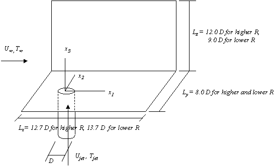
The coordinate system and the geometry of the problem are shown in Fig. 5.1, adapted from (Yuan et al. 1999). The dimensions of the main section vary slightly according to the velocity ratio R, as indicated.
The domain was discretized with 1.34 x 10⁶ control volumes, 45% of them directly downstream of the jet exit. The first control volume next to the jet exit has dimensions of Δx = 0.004D and Δz = 0.006D. These dimensions can be scaled by the shear velocity of the incoming turbulent pipe flow as: Δx+ = 1.4 and Δz+ = 2.2. This resolution ensures that virtually all scales of the fluid are resolved and that the subgrid-scale contributions to the turbulent stresses are negligible near solid surfaces.
The main section inflow velocity profile is fixed as a laminar boundary layer profile with a height of 0.5 D and free stream velocity U∞matching the experimental conditions listed by Sherif & Pletcher (1989). Free slip boundary conditions are prescribed on the lateral and top surfaces and a no-slip condition on the bottom. The inlet plane, the upper wall and the lateral walls were placed at a distance considered sufficient to avoid the imposed boundary conditions to constrain the flow.
As to outflow boundary conditions, the authors tried different schemes and decided that zero gradient condition for all flow variables was the most convenient condition, both simple and effective.
The incoming pipe velocity profile was prescribed at a distance of 1.0D below the flat plate. For a realistic turbulent pipe flow at the inflow boundary, the authors simultaneously ran a second simulation of a temporally evolving pipe flow and extracted instantaneous velocity profiles at each time step. These profiles were then used as velocity boundary conditions at the pipe inflow for the JICF simulation. For the high ReD simulations, the temporal pipe flow simulation was run with a Reτ = 380 while for the low ReD the temporal pipe flow was run with Reτ= 211, where Reτ is a Reynolds number based on the shear velocity of the incoming turbulent pipe flow.
For stability, the fine grids and high velocities led to very small simulation time steps. In consequence, each simulation required approximately 2000 hours on a single processor Cray J90 and approximately 500 hours on a single processor of a Cray C90. The computer time can be evaluated as given by 80 Tu= 80 D/U∞.
Comparisons to experiment
Yuan et al. (1999) made the computations for 3 different cases, to compare results with the experimental data given by Sherif & Pletcher (1989, some times referred to below as SP), with jet radius and Reynolds numbers at the pipe as shown in Table 5.1.
|
| ||
|
|
| |
|
Computational Case 3I |
|
|
|
Computational Case 3II |
|
|
|
Sherif & Pletcher |
|
|
The velocity ratio R was set 3.3 (and not 4.0) to match the centreline velocity of the computational temporal pipe with the experimental centreline velocity given by Sherif & Pletcher. The authors found it necessary to do this adjustment because in the experiments the pipe length was not enough to guarantee fully developed flow in the pipe. A Reynolds number of 4820 was not used by Yuan et al because it would have required significantly more grid points to achieve good flow resolution and, in consequence, more than acceptable computational resources. So, the discrepancies between computed and experimental velocities are explained by the authors as caused by: a) the difference between the experimental jet inflow conditions and b) the fundamentally different cross flow wall boundary layer caused by the lower ReD of the simulations.
Quantities in the centre plane were calculated by Yuan et al (1999) by using the equations:
where ![]() denotes long time average.
denotes long time average.
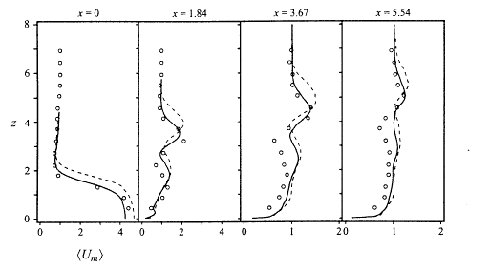
Fig. 5.2 shows vertical profiles of velocity magnitude on the centreplane at four streamwise locations, for cases 3I and 3II. Case 3II profiles seem to match experiment closely, above the point of maximum velocity. Below this point the velocity magnitudes are higher than experiment.
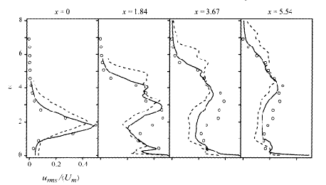
In Fig. 5.3 the authors plot the r.m.s. fluctuations of velocity magnitude defined in the above equations for cases 3I and 3II against the experimental measurements of Sherif & Pletcher. Case 3II compares better with experiment. However, although over the jet exit the agreement between Case 3II and experiment is excellent, at stations downstream r.m.s. magnitudes are underpredicted in the lower half of the profile. A second peak that appears near the wall, particularly at x=1.84 and x=5.54, is explained by fluctuations generated by the wall wake vortices. Through some calculations based on boundary layer theory, the authors show that the higher velocities observed in the lower portions of the velocity profiles are due to differences between the flat plate boundary layers in the simulations and the experiments.
It has been found, both experimentally and computationally that the development of the downstream flow is particularly sensitive to the characteristics of the inflow jet. Different types of inflow conditions have been tried by the authors in cases A, B and C, where they varied the velocity ratio R and the flow condition (Table 5.2).
|
| |||
|
R |
ReD |
Flow condition | |
|
Case A |
4.0 |
1050 |
Plug flow |
|
Case B |
4.0 |
1050 |
Mean turbulent pipe profile |
|
Case C |
4.0 |
1050 |
Temporally evolving pipe |
|
Case 3I |
3.3 |
1050 |
Temporally evolving pipe |
|
Case 3II |
3.3 |
2100 |
Temporally evolving pipe |
For Case A the inflow condition was specified at the level of the flat plate and for the other cases 1 diameter below the level of the flat plate. The velocity magnitude profiles over the jet exit for each case are shown in Fig. 5.4. The worst results are those for Case A. In Case B a 1/7 power law approximation was used to the pipe flow. In Cases 3I and 3II R=3.3 was found to match the experimental data better than R=4.0. The reason seems to be that the experimental arrangements did not allow for a fully developed flow in the pipe, producing a centre line velocity lower than that calculated by the 1/7 power law.
Given the uncertainties in the experiments, particularly with respect to the boundary layer and to the pipe flow, the agreement between calculations and experiments is very good.
Yagci and Kavsaoglu (1993) analysed a swirling subsonic jet injected into a subsonic cross flow, using a three dimensional, thin layer, Reynolds averaged, compressible Navier Stokes solver. The flow and the coordinate system are described in Fig. 5.5, reproduced from the authors.
In the jet region they used the algebraic turbulence model proposed by Oh and Schetz (1990). In other viscous turbulent flow areas they used the Baldwin Lomax turbulence model. Riemann invariants based characteristic boundary conditions have been considered as input boundary conditions for the main flow. At the output they used inverse characteristic boundary conditions. Their test case is the experimental case with 58% swirl, with velocity ratio 4, as described by Kavsaoglu and Schetz (1989).
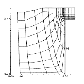
Their grid was obtained by rotation of a two dimensional half grid around the jet axis. The grid had a cavity at the jet entrance. This grid was extended from -15 D to 20 D in the x direction, from -15 D to 15 D in the y direction and from -0.5 D to 15 D in the z direction where D is the jet exit diameter. The size of the grid was 42 x 55 x 45 points, in the x, h, z directions (Figs. 5.6 to 5.8).
At the bottom plane no slip condition was applied from J=6 to J=37 and at the top plane free stream conditions were applied. At the outer surface (J=JMAX) inflow characteristic boundary conditions were applied from K=1 to K=15 and from K=41 to KMAX=55. Outflow (inverse) characteristic boundary conditions were applied from K=16 to K=40. Inflow and outflow boundary conditions are described in detail in this paper and in another paper by Kavsaoglu et al. (1993).
As to the turbulence models, the Baldwin-Lomax model was applied over the flat plate up to z/D = 2.0, excluding the cavity region. The model of Oh and Schetz was applied for the curved jet region. No other turbulence models were applied to other regions, such as the wake behind the jet.
As in the experiments, the velocity ratio was 4 and the Reynolds number based on cross flow velocity and the jet diameter was about 51400. However, the experimental free stream and the jet Mach numbers were respectively 0.05 and 0.2, whilst these Mach numbers have been 0.075 and 0.3 in the calculations. The reason for this is not clear to this writer.
Results for 42 x 55 x 45 grid points were obtained at an IBM 9021-500 vector computer after 6000 iterations, spending 13 seconds per iteration (a total of approximately 22 hours). They found good agreement with the velocity plots of Figs. 4.15 to 4.18 and also with pressure coefficient plots, not reproduced in the current review. As to surface pressures, they found a good agreement in some regions, not so good at the immediate vicinity of the jet exit. They attribute this to grid skewness and / or to turbulence modelling. Due to swirl introducing a strong shear flow in directions not normal to the wall, they argue that a full Navier Stokes solution might be more appropriate than thin layer. A disagreement between the calculated pressure coefficients and the experimental pressure coefficients at the rear of the jet exit was also attributed to turbulence modelling and the authors suggest that a more appropriate model for the wake region is needed.
© copyright ERCOFTAC 2004
Contributors: Flavio Franco - ABB ALSTOM Power UK Ltd


