Stagnation point flow

Underlying Flow Regime 3-12 © copyright ERCOFTAC 2004

Evaluation

Comparison of CFD calculations with Experiments

The following figures are taken from Medic (2001) and Medic and Durbin (2002), where the description is mainly taken from. Four different models (original k-ε, k-ε with T bound, Kato-Launders k-ε v²-f) were used and their respective predictions were compared with measurements.

Figure 1 shows the distribution of the isentropic Mach number M_is along the curvilinear co-ordinate s, normalised by the chord length and the origin placed at the stagnation point. The M_is distribution is not strongly affected by the choice of the turbulence model. The slightly lower values of the original k-ε model can be explained by attributing the excessive k (or ν_t) levels predicted by this model.

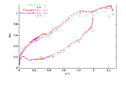
Fig. 1: Isentropic Mach number distribution along pressure and suction side for different turbulence models

The measured and predicted heat transfer coefficient h_t, which is defined as h_t = q_w/(T_0∞ − T_w), along the respective suction and pressure sides of the blade is shown in Figure 2. Significant differences among the various models can be observed here. The original k-ε model strongly over-predicts the heat transfer coefficient, especially on the pressure side towards the trailing edge. The same is reported for the original k-ω model by Medic and Durbin (2002). The levels of the predicted heat transfer by the Kato-Launder formulation or the bound on the turbulent time scale model (T bound) are much closer to the experiments. However, at the leading edge on the suction side h_t is from both models over 30% too high. The predicted slope towards the trailing edge is steeper than from the measurements. On the other hand, the predictions of h_t are better on the pressure side. This indicates the sensitivity of these two models (Kato-Launder and T bound) against an adverse pressure gradient. Of all four models considered in Medic (2001), the v²-f model yields the best results. This model is the only model which is able to capture the trough on the suction side of the experiments. Medic and Durbin (2002) pointed out, that this characteristic is due to the fact that the v²-f model is able to predict a reasonable transition location. However, on the pressure side this model under-predicts the recovery of the heat transfer coefficient towards the trailing edge. This may be caused by the tendency of the model towards relaminarisation of the flow (Medic and Durbin, 2002).

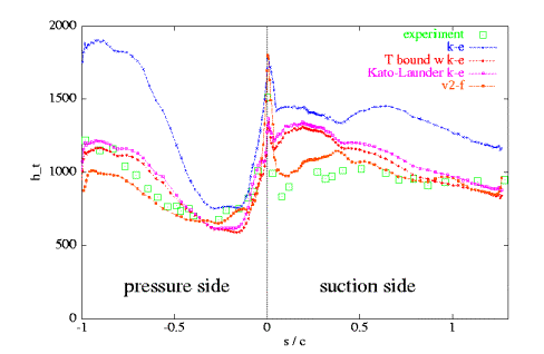
Fig. 2: Heat transfer coefficient h_t distribution along pressure and suction side for different turbulence models

The heat transfer coefficient is related to the eddy viscosity, where the latter quantity is a function of the turbulent kinetic energy k. Therefore, the differences of the prediction of h_t obtained from the different models can be directly linked to k. Figures 3 — 6 show the turbulent kinetic energy distribution predicted by the four considered models. Unfortunately, only computed values of this quantity are presented in Medic and Durbin (2002).

An outstanding feature of these results is that in the centre of the passage the turbulent kinetic energy levels predicted by the original k-ε model (or k-ω model) are about 30 times higher than from the v²-f model. Furthermore, the latter model shows a decrease of turbulent intensity in the centre passage in contrast to the former model.

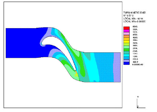
Fig. 3: Iso-lines of turbulent kinetic energy for standard k-ε model.

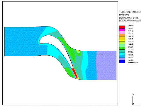
Fig. 4: Iso-lines of turbulent kinetic energy for v²-f model.

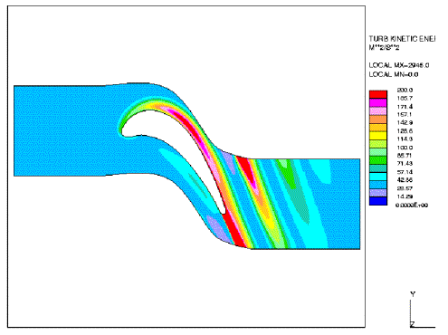
Fig. 5: Iso-lines of turbulent kinetic energy for k-ε model with modification according to Kato-Launder

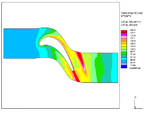
Fig. 6: Iso-lines of turbulent kinetic energy for k-ε model with bound on time scale

Conclusions

In simple cases one-equation models seem to be an option for the turbulence modelling, since these models do not experience a stagnation point anomaly. However, the problem of lack of information of the prescribed length scale restricts the use of one-equation models to a very limited range of cases.

The results from Medic and Durban (2002) suggest that an improvement of the performance of the standard k-ε or k-ω models is possible by using the v²-f model. Other options would be the implementation of a bound on the time scale or modifying the production term in the described manner, i.e. the Kato-Launder modification.

As mentioned above, higher order turbulence models may perform better than eddy-viscosity based models but are often not a practical option for many industrial applications. The recommendation is therefore to use — at least for applications with limited computer resources — models derived from the k-ε or k-ω formulation. Often for industrial purposes not the fine structure of turbulence is of interest, therefore the chosen model should be able to capture the main physical features of the flow field.

Contributors: Beat Ribi - MAN Turbomaschinen AG Schweiz